Quick start guide
In the following we provide some pointers about which functions and classes to use for different problems related to optimal transport (OT) and machine learning. We refer when we can to concrete examples in the documentation that are also available as notebooks on the POT Github.
Note
For a good introduction to numerical optimal transport we refer the reader to the book by Peyré and Cuturi [15]. For more detailed introduction to OT and how it can be used in ML applications we refer the reader to the following OTML tutorial.
Note
Since version 0.8, POT provides a backend to automatically solve some OT problems independently from the toolbox used by the user (numpy/torch/jax). We provide a discussion about which functions are compatible in section Backend section .
Why Optimal Transport ?
When to use OT
Optimal Transport (OT) is a mathematical problem introduced by Gaspard Monge in 1781 that aim at finding the most efficient way to move mass between distributions. The cost of moving a unit of mass between two positions is called the ground cost and the objective is to minimize the overall cost of moving one mass distribution onto another one. The optimization problem can be expressed for two distributions \(\mu_s\) and \(\mu_t\) as
where \(c(\cdot,\cdot)\) is the ground cost and the constraint \(m \# \mu_s = \mu_t\) ensures that \(\mu_s\) is completely transported to \(\mu_t\). This problem is particularly difficult to solve because of this constraint and has been replaced in practice (on discrete distributions) by a linear program easier to solve. It corresponds to the Kantorovitch formulation where the Monge mapping \(m\) is replaced by a joint distribution (OT matrix expressed in the next section) (see Solving optimal transport).
From the optimization problem above we can see that there are two main aspects to the OT solution that can be used in practical applications:
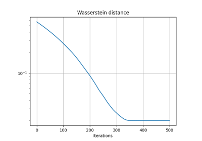
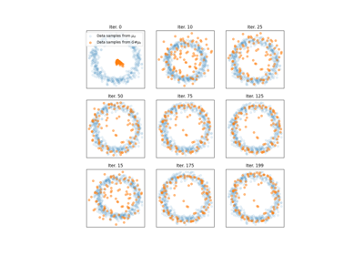
The optimal value (Wasserstein distance): Measures similarity between distributions.
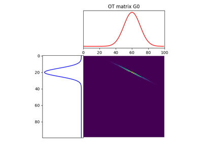
The optimal mapping (Monge mapping, OT matrix): Finds correspondences between distributions.
In the first case, OT can be used to measure similarity between distributions (or datasets), in this case the Wasserstein distance (the optimal value of the problem) is used. In the second case one can be interested in the way the mass is moved between the distributions (the mapping). This mapping can then be used to transfer knowledge between distributions.
Wasserstein distance between distributions
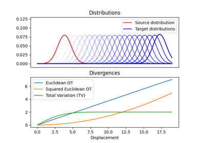
OT is often used to measure similarity between distributions, especially when they do not share the same support. When the support between the distributions is disjoint OT-based Wasserstein distances compare favorably to popular f-divergences including the popular Kullback-Leibler, Jensen-Shannon divergences, and the Total Variation distance. What is particularly interesting for data science applications is that one can compute meaningful sub-gradients of the Wasserstein distance. For these reasons it became a very efficient tool for machine learning applications that need to measure and optimize similarity between empirical distributions.
Numerous contributions make use of this an approach is the machine learning (ML) literature. For example OT was used for training Generative Adversarial Networks (GANs) in order to overcome the vanishing gradient problem. It has also been used to find discriminant or robust subspaces for a dataset. The Wasserstein distance has also been used to measure similarity between word embeddings of documents or between signals or spectra.
OT for mapping estimation
A very interesting aspect of OT problem is the OT mapping in itself. When computing optimal transport between discrete distributions one output is the OT matrix that will provide you with correspondences between the samples in each distributions.
This correspondence is estimated with respect to the OT criterion and is found in a non-supervised way, which makes it very interesting on problems of transfer between datasets. It has been used to perform color transfer between images or in the context of domain adaptation. More recent applications include the use of extension of OT (Gromov-Wasserstein) to find correspondences between languages in word embeddings.
When to use POT
The main objective of POT is to provide OT solvers for the rapidly growing area of OT in the context of machine learning. To this end we implement a number of solvers that have been proposed in research papers. Doing so we aim to promote reproducible research and foster novel developments.
One very important aspect of POT is its ability to be easily extended. For
instance we provide a very generic OT solver ot.optim.cg that can solve
OT problems with any smooth/continuous regularization term making it
particularly practical for research purpose. Note that this generic solver has
been used to solve both graph Laplacian regularization OT and Gromov
Wasserstein [30].
When not to use POT
While POT has to the best of our knowledge one of the most efficient exact OT solvers, it has not been designed to handle large scale OT problems. For instance the memory cost for an OT problem is always \(\mathcal{O}(n^2)\) in memory because the cost matrix has to be computed. The exact solver in of time complexity \(\mathcal{O}(n^3\log(n))\) and the Sinkhorn solver has been proven to be nearly \(\mathcal{O}(n^2)\) which is still too complex for very large scale solvers.
If you need to solve OT with large number of samples, we recommend to use entropic regularization and memory efficient implementation of Sinkhorn as proposed in GeomLoss. This implementation is compatible with Pytorch and can handle large number of samples. Another approach to estimate the Wasserstein distance for very large number of sample is to use the trick from Wasserstein GAN that solves the problem in the dual with a neural network estimating the dual variable. Note that in this case you are only solving an approximation of the Wasserstein distance because the 1-Lipschitz constraint on the dual cannot be enforced exactly (approximated through filter thresholding or regularization). Finally note that in order to avoid solving large scale OT problems, a number of recent approached minimized the expected Wasserstein distance on minibatches that is different from the Wasserstein but has better computational and statistical properties.
Optimal transport and Wasserstein distance
Note
In POT, most functions that solve OT or regularized OT problems have two
versions that return the OT matrix or the value of the optimal solution. For
instance ot.emd returns the OT matrix and ot.emd2 returns the
Wasserstein distance. This approach has been implemented in practice for all
solvers that return an OT matrix (even Gromov-Wasserstein).
Solving optimal transport
The optimal transport problem between discrete distributions is often expressed as
where:
\(M\in\mathbb{R}_+^{m\times n}\) is the metric cost matrix defining the cost to move mass from bin \(a_i\) to bin \(b_j\).
\(a\) and \(b\) are histograms on the simplex (positive, sum to 1) that represent the weights of each samples in the source an target distributions.
Solving the linear program above can be done using the function ot.emd
that will return the optimal transport matrix \(\gamma^*\):
# a and b are 1D histograms (sum to 1 and positive)
# M is the ground cost matrix
T = ot.emd(a, b, M)  # exact linear program
The method implemented for solving the OT problem is the network simplex. It is implemented in C from [1]. It has a complexity of \(O(n^3)\) but the solver is quite efficient and uses sparsity of the solution.
Examples of use for ot.emd
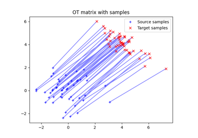
Optimal Transport between 2D empirical distributions
Computing Wasserstein distance
The value of the OT solution is often more interesting than the OT matrix:
It can computed from an already estimated OT matrix with
np.sum(T*M) or directly with the function ot.emd2.
# a and b are 1D histograms (sum to 1 and positive)
# M is the ground cost matrix
W = ot.emd2(a, b, M)  # Wasserstein distance / EMD value
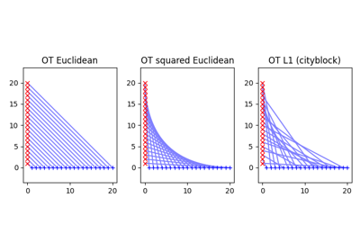
Note that the well known Wasserstein distance between distributions a and b is defined as
\[ \begin{align}\begin{aligned}W_p(a,b)=(\min_{\gamma \in \mathbb{R}_+^{m\times n}} \sum_{i,j}\gamma_{i,j}\|x_i-y_j\|_p)^\frac{1}{p}\\s.t. \gamma 1 = a; \gamma^T 1= b; \gamma\geq 0\end{aligned}\end{align} \]
This means that if you want to compute the \(W_2\) you need to compute the
square root of ot.emd2 when providing
M = ot.dist(xs, xt), that uses the squared euclidean distance by default. Computing
the \(W_1\) Wasserstein distance can be done directly with ot.emd2
when providing M = ot.dist(xs, xt, metric='euclidean') to use the Euclidean
distance.
Examples of use for ot.emd2
Special cases
Note that the OT problem and the corresponding Wasserstein distance can in some special cases be computed very efficiently.
For instance when the samples are in 1D, then the OT problem can be solved in
\(O(n\log(n))\) by using a simple sorting. In this case we provide the
function ot.emd_1d and ot.emd2_1d to return respectively the OT
matrix and value. Note that since the solution is very sparse the sparse
parameter of ot.emd_1d allows for solving and returning the solution for
very large problems. Note that in order to compute directly the \(W_p\)
Wasserstein distance in 1D we provide the function ot.wasserstein_1d that
takes p as a parameter.
Another special case for estimating OT and Monge mapping is between Gaussian
distributions. In this case there exists a close form solution given in Remark
2.29 in [15] and the Monge mapping is an affine function and can be
also computed from the covariances and means of the source and target
distributions. In the case when the finite sample dataset is supposed Gaussian,
we provide ot.gaussian.bures_wasserstein_mapping that returns the parameters for the
Monge mapping.
Regularized Optimal Transport
Recent developments have shown the interest of regularized OT both in terms of computational and statistical properties. We address in this section the regularized OT problems that can be expressed as
where :
\(M\in\mathbb{R}_+^{m\times n}\) is the metric cost matrix defining the cost to move mass from bin \(a_i\) to bin \(b_j\).
\(a\) and \(b\) are histograms (positive, sum to 1) that represent the weights of each samples in the source an target distributions.
\(\Omega\) is the regularization term.
We discuss in the following specific algorithms that can be used depending on the regularization term.
Entropic regularized OT
This is the most common regularization used for optimal transport. It has been proposed in the ML community by Marco Cuturi in his seminal paper [2]. This regularization has the following expression
The use of the regularization term above in the optimization problem has a very
strong impact. First it makes the problem smooth which leads to new optimization
procedures such as the well known Sinkhorn algorithm [2] or L-BFGS (see
ot.smooth ). Next it makes the problem
strictly convex meaning that there will be a unique solution. Finally the
solution of the resulting optimization problem can be expressed as:
where \(u\) and \(v\) are vectors and \(K=\exp(-M/\lambda)\) where the \(\exp\) is taken component-wise. In order to solve the optimization problem, one can use an alternative projection algorithm called Sinkhorn-Knopp that can be very efficient for large values of regularization.
The Sinkhorn-Knopp algorithm is implemented in ot.sinkhorn and
ot.sinkhorn2 that return respectively the OT matrix and the value of the
linear term. Note that the regularization parameter \(\lambda\) in the
equation above is given to those functions with the parameter reg.
>>> import ot
>>> a = [.5, .5]
>>> b = [.5, .5]
>>> M = [[0., 1.], [1., 0.]]
>>> ot.sinkhorn(a, b, M, 1)
array([[ 0.36552929,  0.13447071],
    [ 0.13447071,  0.36552929]])
More details about the algorithms used are given in the following note.
Note
The main function to solve entropic regularized OT is ot.sinkhorn.
This function is a wrapper and the parameter method allows you to select
the actual algorithm used to solve the problem:
method='sinkhorn'callsot.bregman.sinkhorn_knoppthe classic algorithm [2].method='sinkhorn_log'callsot.bregman.sinkhorn_logthe sinkhorn algorithm in log space [2] that is more stable but can be slower in numpy since logsumexp is not implemented in parallel. It is the recommended solver for applications that requires differentiability with a small number of iterations.method='sinkhorn_stabilized'callsot.bregman.sinkhorn_stabilizedthe log stabilized version of the algorithm [9].method='sinkhorn_epsilon_scaling'callsot.bregman.sinkhorn_epsilon_scalingthe epsilon scaling version of the algorithm [9].method='greenkhorn'callsot.bregman.greenkhornthe greedy Sinkhorn version of the algorithm [22].method='screenkhorn'callsot.bregman.screenkhornthe screening sinkhorn version of the algorithm [26].
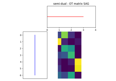
In addition to all those variants of Sinkhorn, we have another
implementation solving the problem in the smooth dual or semi-dual in
ot.smooth. This solver uses the scipy.optimize.minimize
function to solve the smooth problem with L-BFGS-B algorithm. Tu use
this solver, use functions ot.smooth.smooth_ot_dual or
ot.smooth.smooth_ot_semi_dual with parameter reg_type='kl' to
choose entropic/Kullbach-Leibler regularization.
Choosing a Sinkhorn solver
By default and when using a regularization parameter that is not too small
the default Sinkhorn solver should be enough. If you need to use a small
regularization to get sharper OT matrices, you should use the
ot.bregman.sinkhorn_stabilized solver that will avoid numerical
errors. This last solver can be very slow in practice and might not even
converge to a reasonable OT matrix in a finite time. This is why
ot.bregman.sinkhorn_epsilon_scaling that relies on iterating the value
of the regularization (and using warm start) sometimes leads to better
solutions. Note that the greedy version of the Sinkhorn
ot.bregman.greenkhorn can also lead to a speedup and the screening
version of the Sinkhorn ot.bregman.screenkhorn aim a providing a
fast approximation of the Sinkhorn problem. For use of GPU and gradient
computation with small number of iterations we strongly recommend the
ot.bregman.sinkhorn_log solver that will no need to check for
numerical problems.
Recently Genevay et al. [23] introduced the Sinkhorn divergence that build from entropic
regularization to compute fast and differentiable geometric divergence between
empirical distributions. Note that we provide a function that computes directly
(with no need to precompute the M matrix)
the Sinkhorn divergence for empirical distributions in
ot.bregman.empirical_sinkhorn_divergence. Similarly one can compute the
OT matrix and loss for empirical distributions with respectively
ot.bregman.empirical_sinkhorn and ot.bregman.empirical_sinkhorn2.
Finally note that we also provide in ot.stochastic several implementation
of stochastic solvers for entropic regularized OT [18] [19]. Those pure Python
implementations are not optimized for speed but provide a robust implementation
of algorithms in [18] [19].
Examples of use for ot.sinkhorn
Optimal Transport between 2D empirical distributions
Examples of use for ot.sinkhorn2
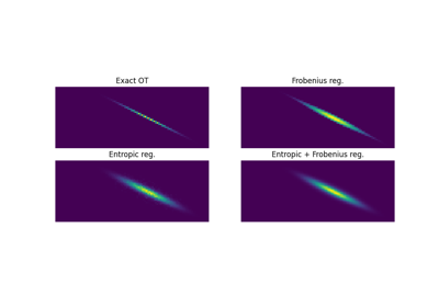
Other regularizations
While entropic OT is the most common and favored in practice, there exists other
kinds of regularizations. We provide in POT two specific solvers for other
regularization terms, namely quadratic regularization and group Lasso
regularization. But we also provide in ot.optim two generic solvers
that allows solving any smooth regularization in practice.
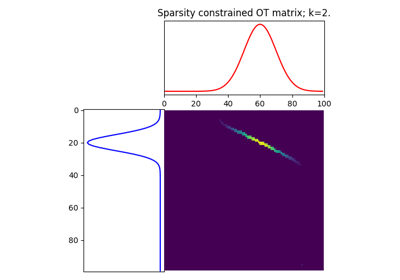
Quadratic regularization
The first general regularization term we can solve is the quadratic regularization of the form
This regularization term has an effect similar to entropic regularization by
densifying the OT matrix, yet it keeps some sort of sparsity that is lost with
entropic regularization as soon as \(\lambda>0\) [17]. This problem can be
solved with POT using solvers from ot.smooth, more specifically
functions ot.smooth.smooth_ot_dual or
ot.smooth.smooth_ot_semi_dual with parameter reg_type='l2' to
choose the quadratic regularization.
Examples of use of quadratic regularization
Group Lasso regularization
Another regularization that has been used in recent years [5] is the group Lasso regularization
where \(\mathcal{G}\) contains non-overlapping groups of lines in the OT
matrix. This regularization proposed in [5] promotes sparsity at the group level and for
instance will force target samples to get mass from a small number of groups.
Note that the exact OT solution is already sparse so this regularization does
not make sense if it is not combined with entropic regularization. Depending on
the choice of p and q, the problem can be solved with different
approaches. When q=1 and p<1 the problem is non-convex but can
be solved using an efficient majoration minimization approach with
ot.sinkhorn_lpl1_mm. When q=2 and p=1 we recover the
convex group lasso and we provide a solver using generalized conditional
gradient algorithm [7] in function ot.da.sinkhorn_l1l2_gl.
Examples of group Lasso regularization
OT for domain adaptation on empirical distributions
Generic solvers
Finally we propose in POT generic solvers that can be used to solve any regularization as long as you can provide a function computing the regularization and a function computing its gradient (or sub-gradient).
In order to solve
you can use function ot.optim.cg that will use a conditional gradient as
proposed in [6] . You need to provide the regularization function as parameter
f and its gradient as parameter df. Note that the conditional gradient relies on
iterative solving of a linearization of the problem using the exact
ot.emd so it can be quite slow in practice. However, being an interior point
algorithm, it always returns a transport matrix that does not violates the marginals.
Another generic solver is proposed to solve the problem:
where \(\Omega_e\) is the entropic regularization. In this case we use a
generalized conditional gradient [7] implemented in ot.optim.gcg that
does not linearize the entropic term but
relies on ot.sinkhorn for its iterations.
Examples of the generic solvers
Wasserstein Barycenters
A Wasserstein barycenter is a distribution that minimizes its Wasserstein distance with respect to other distributions [16]. It corresponds to minimizing the following problem by searching a distribution \(\mu\) such that
In practice we model a distribution with a finite number of support position:
where \(a\) is an histogram on the simplex and the \(\{x_i\}\) are the position of the support. We can clearly see here that optimizing \(\mu\) can be done by searching for optimal weights \(a\) or optimal support \(\{x_i\}\) (optimizing both is also an option). We provide in POT solvers to estimate a discrete Wasserstein barycenter in both cases.
Barycenters with fixed support
When optimizing a barycenter with a fixed support, the optimization problem can be expressed as
where \(b_k\) are also weights in the simplex. In the non-regularized case,
the problem above is a classical linear program. In this case we propose a
solver ot.lp.barycenter() that relies on generic LP solvers. By default the
function uses scipy.optimize.linprog, but more efficient LP solvers from
cvxopt can be also used by changing parameter solver. Note that this problem
requires to solve a very large linear program and can be very slow in
practice.
Similarly to the OT problem, OT barycenters can be computed in the regularized
case. When entropic regularization is used, the problem can be solved with a
generalization of the Sinkhorn algorithm based on Bregman projections [3]. This
algorithm is provided in function ot.bregman.barycenter also available as
ot.barycenter. In this case, the algorithm scales better to large
distributions and relies only on matrix multiplications that can be performed in
parallel.
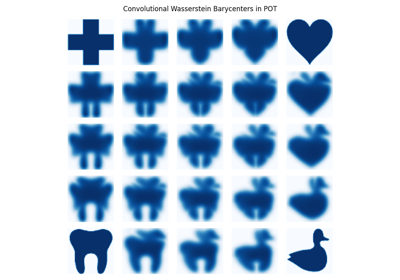
In addition to the speedup brought by regularization, one can also greatly
accelerate the estimation of Wasserstein barycenter when the support has a
separable structure [21]. In the case of 2D images for instance one can replace
the matrix vector production in the Bregman projections by convolution
operators. We provide an implementation of this algorithm in function
ot.bregman.convolutional_barycenter2d.
Examples of Wasserstein and regularized Wasserstein barycenters
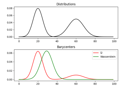
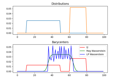
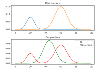
1D Wasserstein barycenter: exact LP vs entropic regularization
1D Wasserstein barycenter: exact LP vs entropic regularization
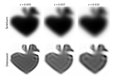
An example of convolutional barycenter (ot.bregman.convolutional_barycenter2d) computation
Barycenters with free support
Estimating the Wasserstein barycenter with free support but fixed weights corresponds to solving the following optimization problem:
We provide a solver based on [20] in
ot.lp.free_support_barycenter. This function minimize the problem and
return a locally optimal support \(\{x_i\}\) for uniform or given weights
\(a\).
Examples of free support barycenter estimation
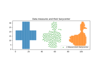
2D free support Wasserstein barycenters of distributions
Monge mapping and Domain adaptation
The original transport problem investigated by Gaspard Monge was seeking for a
mapping function that maps (or transports) between a source and target
distribution but that minimizes the transport loss. The existence and uniqueness of this
optimal mapping is still an open problem in the general case but has been proven
for smooth distributions by Brenier in his eponym theorem. We provide in
ot.da several solvers for smooth Monge mapping estimation and domain
adaptation from discrete distributions.
Monge Mapping estimation
We now discuss several approaches that are implemented in POT to estimate or approximate a Monge mapping from finite distributions.
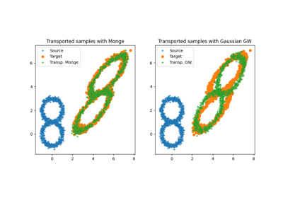
First note that when the source and target distributions are supposed to be Gaussian
distributions, there exists a close form solution for the mapping and its an
affine function [14] of the form \(T(x)=Ax+b\) . In this case we provide the function
ot.gaussian.bures_wasserstein_mapping that returns the operator \(A\) and vector
\(b\). Note that if the number of samples is too small there is a parameter
reg that provides a regularization for the covariance matrix estimation.
For a more general mapping estimation we also provide the barycentric mapping
proposed in [6]. It is implemented in the class ot.da.EMDTransport and
other transport-based classes in ot.da . Those classes are discussed more
in the following but follow an interface similar to scikit-learn classes. Finally a
method proposed in [8] that estimates a continuous mapping approximating the
barycentric mapping is provided in ot.da.joint_OT_mapping_linear for
linear mapping and ot.da.joint_OT_mapping_kernel for non-linear mapping.
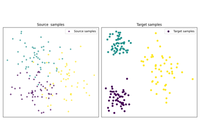
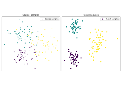
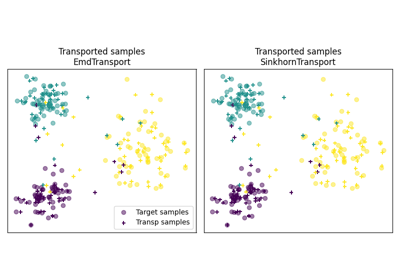
Domain adaptation classes
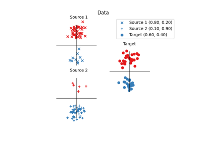
The use of OT for domain adaptation (OTDA) has been first proposed in [5] that also introduced the group Lasso regularization. The main idea of OTDA is to estimate a mapping of the samples between source and target distributions which allows to transport labeled source samples onto the target distribution with no labels.
We provide several classes based on ot.da.BaseTransport that provide
several OT and mapping estimations. The interface of those classes is similar to
classifiers in scikit-learn. At initialization, several parameters such as
regularization parameter value can be set. Then one needs to estimate the
mapping with function ot.da.BaseTransport.fit. Finally one can map the
samples from source to target with ot.da.BaseTransport.transform and
from target to source with ot.da.BaseTransport.inverse_transform.
Here is an example for class ot.da.EMDTransport:
ot_emd = ot.da.EMDTransport()
ot_emd.fit(Xs=Xs, Xt=Xt)
Xs_mapped = ot_emd.transform(Xs=Xs)
A list of the provided implementation is given in the following note.
Note
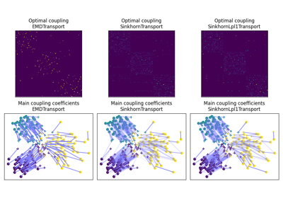
Here is a list of the OT mapping classes inheriting from
ot.da.BaseTransport
ot.da.EMDTransport: Barycentric mapping with EMD transportot.da.SinkhornTransport: Barycentric mapping with Sinkhorn transportot.da.SinkhornL1l2Transport: Barycentric mapping with Sinkhorn + group Lasso regularization [5]ot.da.SinkhornLpl1Transport: Barycentric mapping with Sinkhorn + non convex group Lasso regularization [5]ot.da.LinearTransport: Linear mapping estimation between Gaussians [14]ot.da.MappingTransport: Nonlinear mapping estimation [8]
Examples of the use of OTDA classes
OT with Laplacian regularization for domain adaptation
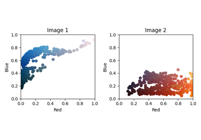
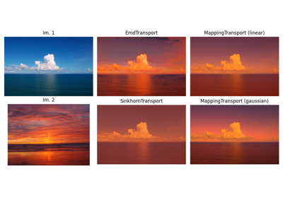
OT for image color adaptation with mapping estimation
OT for domain adaptation on empirical distributions
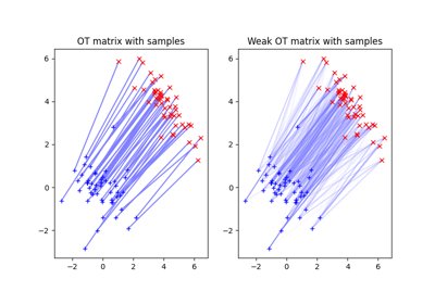
Unbalanced and partial OT
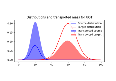
Unbalanced optimal transport
Unbalanced OT is a relaxation of the entropy regularized OT problem where the violation of the constraint on the marginals is added to the objective of the optimization problem. The unbalanced OT metric between two unbalanced histograms a and b is defined as [25] [10]:
where KL is the Kullback-Leibler divergence. This formulation allows for
computing approximate mapping between distributions that do not have the same
amount of mass. Interestingly the problem can be solved with a generalization of
the Bregman projections algorithm [10]. We provide a solver for unbalanced OT
in ot.unbalanced. Computing the optimal transport
plan or the transport cost is similar to the balanced case. The Sinkhorn-Knopp
algorithm is implemented in ot.sinkhorn_unbalanced and ot.sinkhorn_unbalanced2
that return respectively the OT matrix and the value of the
linear term.
Note
The main function to solve entropic regularized UOT is ot.sinkhorn_unbalanced.
This function is a wrapper and the parameter method helps you select
the actual algorithm used to solve the problem:
method='sinkhorn'callsot.unbalanced.sinkhorn_knopp_unbalancedthe generalized Sinkhorn algorithm [25] [10].method='sinkhorn_stabilized'callsot.unbalanced.sinkhorn_stabilized_unbalancedthe log stabilized version of the algorithm [10].
Examples of Unbalanced OT
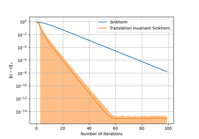
Translation Invariant Sinkhorn for Unbalanced Optimal Transport
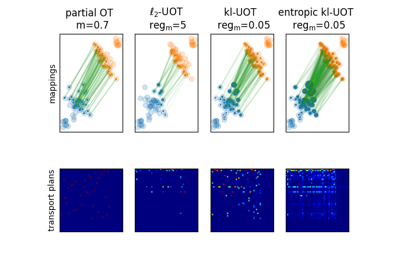
2D examples of exact and entropic unbalanced optimal transport
Unbalanced Barycenters
As with balanced distributions, we can define a barycenter of a set of histograms with different masses as a Fréchet Mean:
\[\min_{\mu} \quad \sum_{k} w_kW_u(\mu,\mu_k)\]
where \(W_u\) is the unbalanced Wasserstein metric defined above. This problem
can also be solved using generalized version of Sinkhorn’s algorithm and it is
implemented the main function ot.barycenter_unbalanced.
Note
The main function to compute UOT barycenters is ot.barycenter_unbalanced.
This function is a wrapper and the parameter method helps you select
the actual algorithm used to solve the problem:
method='sinkhorn'callsot.unbalanced.barycenter_unbalanced_sinkhorn_unbalanced()the generalized Sinkhorn algorithm [10].method='sinkhorn_stabilized'callsot.unbalanced.barycenter_unbalanced_stabilizedthe log stabilized version of the algorithm [10].
Examples of Unbalanced OT barycenters
1D Wasserstein barycenter demo for Unbalanced distributions
Partial optimal transport
Partial OT is a variant of the optimal transport problem when only a fixed amount of mass m is to be transported. The partial OT metric between two histograms a and b is defined as [28]:
Interestingly the problem can be casted into a regular OT problem by adding reservoir points
in which the surplus mass is sent [29]. We provide a solver for partial OT
in ot.partial. The exact resolution of the problem is computed in ot.partial.partial_wasserstein
and ot.partial.partial_wasserstein2 that return respectively the OT matrix and the value of the
linear term. The entropic solution of the problem is computed in ot.partial.entropic_partial_wasserstein
(see [3]).
The partial Gromov-Wasserstein formulation of the problem
is computed in ot.partial.partial_gromov_wasserstein and in
ot.partial.entropic_partial_gromov_wasserstein when considering the entropic
regularization of the problem.
Examples of Partial OT
2D examples of exact and entropic unbalanced optimal transport
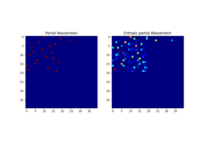
Partial Wasserstein and Gromov-Wasserstein example
Gromov Wasserstein and extensions
Gromov Wasserstein(GW)
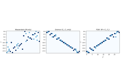
Gromov Wasserstein (GW) is a generalization of OT to distributions that do not lie in the same space [13]. In this case one cannot compute distance between samples from the two distributions. [13] proposed instead to realign the metric spaces by computing a transport between distance matrices. The Gromov Wasserstein alignment between two distributions can be expressed as the one minimizing:
where :\(C1\) is the distance matrix between samples in the source
distribution and \(C2\) the one between samples in the target,
\(L(C1_{i,k},C2_{j,l})\) is a measure of similarity between
\(C1_{i,k}\) and \(C2_{j,l}\) often chosen as
\(L(C1_{i,k},C2_{j,l})=\|C1_{i,k}-C2_{j,l}\|^2\). The optimization problem
above is a non-convex quadratic program but we provide a solver that finds a
local minimum using conditional gradient in ot.gromov.gromov_wasserstein.
There also exists an entropic regularized variant of GW that has been proposed in
[12] and we provide an implementation of their algorithm in
ot.gromov.entropic_gromov_wasserstein.
Examples of computation of GW, regularized G and FGW
Gromov Wasserstein barycenters
Note that similarly to Wasserstein distance GW allows for the definition of GW barycenters that can be expressed as
where \(Ck\) is the distance matrix between samples in distribution
\(k\). Note that interestingly the barycenter is defined as a symmetric
positive matrix. We provide a block coordinate optimization procedure in
ot.gromov.gromov_barycenters and
ot.gromov.entropic_gromov_barycenters for non-regularized and regularized
barycenters respectively.
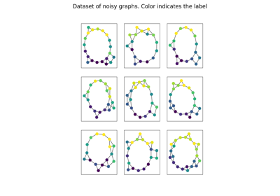
Finally note that recently a fusion between Wasserstein and GW, coined Fused
Gromov-Wasserstein (FGW) has been proposed [24].
It allows to compute a similarity between objects that are only partly in
the same space. As such it can be used to measure similarity between labeled
graphs for instance and also provide computable barycenters.
The implementations of FGW and FGW barycenter is provided in functions
ot.gromov.fused_gromov_wasserstein and ot.gromov.fgw_barycenters.
Examples of GW, regularized G and FGW barycenters
Other applications
We discuss in the following several OT related problems and tools that has been proposed in the OT and machine learning community.
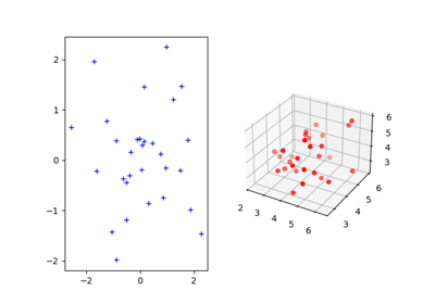
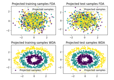
Wasserstein Discriminant Analysis
Wasserstein Discriminant Analysis [11] is a generalization of Fisher Linear Discriminant Analysis that allows discrimination between classes that are not linearly separable. It consists in finding a linear projector optimizing the following criterion
where \(\#\) is the push-forward operator, \(OT_e\) is the entropic OT
loss and \(\mu_i\) is the
distribution of samples from class \(i\). \(P\) is also constrained to
be in the Stiefel manifold. WDA can be solved in POT using function
ot.dr.wda. It requires to have installed pymanopt and
autograd for manifold optimization and automatic differentiation
respectively. Note that we also provide the Fisher discriminant estimator in
ot.dr.fda for easy comparison.
Warning
Note that due to the hard dependency on pymanopt and
autograd, ot.dr is not imported by default. If you want to
use it you have to specifically import it with import ot.dr .
Examples of the use of WDA
Solving OT with Multiple backends on CPU/GPU
Since version 0.8, POT provides a backend that allows to code solvers independently from the type of the input arrays. The idea is to provide the user with a package that works seamlessly and returns a solution for instance as a Pytorch tensors when the function has Pytorch tensors as input.
How it works
The aim of the backend is to use the same function independently of the type of the input arrays.
For instance when executing the following code
# a and b are 1D histograms (sum to 1 and positive)
# M is the ground cost matrix
T = ot.emd(a, b, M)  # exact linear program
w = ot.emd2(a, b, M)  # Wasserstein computation
the functions ot.emd and ot.emd2 can take inputs of the type
numpy.array, torch.tensor or jax.numpy.array. The output of
the function will be the same type as the inputs and on the same device. When
possible all computations are done on the same device and also when possible the
output will be differentiable with respect to the input of the function.
GPU acceleration
The backends provide automatic computations/compatibility on GPU for most of the POT functions. Note that all solvers relying on the exact OT solver en C++ will need to solve the problem on CPU which can incur some memory copy overhead and be far from optimal when all other computations are done on GPU. They will still work on array on GPU since the copy is done automatically.
Some of the functions that rely on the exact C++ solver are:
List of compatible Backends
Numpy (all functions and solvers)
Pytorch (all outputs differentiable w.r.t. inputs)
Jax (Some functions are differentiable some require a wrapper)
Tensorflow (all outputs differentiable w.r.t. inputs)
Cupy (no differentiation, GPU only)
The library automatically detects which backends are available for use. A backend is instantiated lazily only when necessary to prevent unwarranted GPU memory allocations. You can also disable the import of a specific backend library (e.g., to accelerate loading of ot library) using the environment variable POT_BACKEND_DISABLE_<NAME> with <NAME> in (TORCH,TENSORFLOW,CUPY,JAX). For instance, to disable TensorFlow, set export POT_BACKEND_DISABLE_TENSORFLOW=1. It’s important to note that the numpy backend cannot be disabled.
List of compatible modules
This list will get longer for new releases and will hopefully disappear when POT become fully implemented with the backend.
FAQ
How to solve a discrete optimal transport problem ?
The solver for discrete OT is the function
ot.emdthat returns the OT transport matrix. If you want to solve a regularized OT you can useot.sinkhorn.Here is a simple use case:
# a and b are 1D histograms (sum to 1 and positive)
# M is the ground cost matrix
T = ot.emd(a, b, M)  # exact linear program
T_reg = ot.sinkhorn(a, b, M, reg)  # entropic regularized OT
More detailed examples can be seen on this example: Optimal Transport between 2D empirical distributions
pip install POT fails with error : ImportError: No module named Cython.Build
As discussed shortly in the README file. POT<0.8 requires to have
numpyandcythoninstalled to build. This corner case is not yet handled bypipand for now you need to install both library prior to installing POT.Note that this problem do not occur when using conda-forge since the packages there are pre-compiled.
See Issue #59 for more details.
Why is Sinkhorn slower than EMD ?
This might come from the choice of the regularization term. The speed of convergence of Sinkhorn depends directly on this term [22]. When the regularization gets very small the problem tries to approximate the exact OT which leads to slow convergence in addition to numerical problems. In other words, for large regularization Sinkhorn will be very fast to converge, for small regularization (when you need an OT matrix close to the true OT), it might be quicker to use the EMD solver.
Also note that the numpy implementation of Sinkhorn can use parallel computation depending on the configuration of your system, yet very important speedup can be obtained by using a GPU implementation since all operations are matrix/vector products.