Note
Go to the end to download the full example code.
Wasserstein 2 Minibatch GAN with PyTorch
Note
Example added in release: 0.8.0.
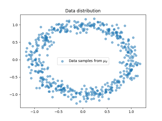
In this example we train a Wasserstein GAN using Wasserstein 2 on minibatches as a distribution fitting term.
We want to train a generator \(G_\theta\) that generates realistic data from random noise drawn form a Gaussian \(\mu_n\) distribution so that the data is indistinguishable from true data in the data distribution \(\mu_d\). To this end Wasserstein GAN [Arjovsky2017] aim at optimizing the parameters \(\theta\) of the generator with the following optimization problem:
In practice we do not have access to the full distribution \(\mu_d\) but samples and we cannot compute the Wasserstein distance for large dataset. [Arjovsky2017] proposed to approximate the dual potential of Wasserstein 1 with a neural network recovering an optimization problem similar to GAN. In this example we will optimize the expectation of the Wasserstein distance over minibatches at each iterations as proposed in [Genevay2018]. Optimizing the Minibatches of the Wasserstein distance has been studied in [Fatras2019].
[Arjovsky2017] Arjovsky, M., Chintala, S., & Bottou, L. (2017, July). Wasserstein generative adversarial networks. In International conference on machine learning (pp. 214-223). PMLR.
[Genevay2018] Genevay, Aude, Gabriel Peyré, and Marco Cuturi. “Learning generative models with sinkhorn divergences.” International Conference on Artificial Intelligence and Statistics. PMLR, 2018.
[Fatras2019] Fatras, K., Zine, Y., Flamary, R., Gribonval, R., & Courty, N. (2020, June). Learning with minibatch Wasserstein: asymptotic and gradient properties. In the 23nd International Conference on Artificial Intelligence and Statistics (Vol. 108).
# Author: Remi Flamary <remi.flamary@polytechnique.edu>
#
# License: MIT License
# sphinx_gallery_thumbnail_number = 3
import numpy as np
import matplotlib.pyplot as pl
import matplotlib.animation as animation
import torch
from torch import nn
import ot
Data generation
torch.manual_seed(1)
sigma = 0.1
n_dims = 2
n_features = 2
def get_data(n_samples):
c = torch.rand(size=(n_samples, 1))
angle = c * 2 * np.pi
x = torch.cat((torch.cos(angle), torch.sin(angle)), 1)
x += torch.randn(n_samples, 2) * sigma
return x
Plot data
/home/circleci/project/examples/backends/plot_wass2_gan_torch.py:87: SyntaxWarning: invalid escape sequence '\m'
pl.scatter(x[:, 0], x[:, 1], label="Data samples from $\mu_d$", alpha=0.5)
<matplotlib.legend.Legend object at 0x7e974d786240>
Generator Model
# define the MLP model
class Generator(torch.nn.Module):
def __init__(self):
super(Generator, self).__init__()
self.fc1 = nn.Linear(n_features, 200)
self.fc2 = nn.Linear(200, 500)
self.fc3 = nn.Linear(500, n_dims)
self.relu = torch.nn.ReLU() # instead of Heaviside step fn
def forward(self, x):
output = self.fc1(x)
output = self.relu(output) # instead of Heaviside step fn
output = self.fc2(output)
output = self.relu(output)
output = self.fc3(output)
return output
Training the model
G = Generator()
optimizer = torch.optim.RMSprop(G.parameters(), lr=0.00019, eps=1e-5)
# number of iteration and size of the batches
n_iter = 200 # set to 200 for doc build but 1000 is better ;)
size_batch = 500
# generate statis samples to see their trajectory along training
n_visu = 100
xnvisu = torch.randn(n_visu, n_features)
xvisu = torch.zeros(n_iter, n_visu, n_dims)
ab = torch.ones(size_batch) / size_batch
losses = []
for i in range(n_iter):
# generate noise samples
xn = torch.randn(size_batch, n_features)
# generate data samples
xd = get_data(size_batch)
# generate sample along iterations
xvisu[i, :, :] = G(xnvisu).detach()
# generate samples and compte distance matrix
xg = G(xn)
M = ot.dist(xg, xd)
loss = ot.emd2(ab, ab, M)
losses.append(float(loss.detach()))
if i % 10 == 0:
print("Iter: {:3d}, loss={}".format(i, losses[-1]))
loss.backward()
optimizer.step()
optimizer.zero_grad()
del M
pl.figure(2)
pl.semilogy(losses)
pl.grid()
pl.title("Wasserstein distance")
pl.xlabel("Iterations")
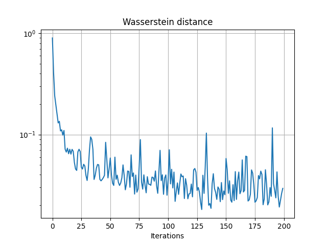
Iter: 0, loss=0.9009847640991211
Iter: 10, loss=0.10964284837245941
Iter: 20, loss=0.04564394801855087
Iter: 30, loss=0.03516071289777756
Iter: 40, loss=0.05013977363705635
Iter: 50, loss=0.058588504791259766
Iter: 60, loss=0.03730057179927826
Iter: 70, loss=0.04171676188707352
Iter: 80, loss=0.03168988972902298
Iter: 90, loss=0.031197285279631615
Iter: 100, loss=0.03596879169344902
Iter: 110, loss=0.03272819146513939
Iter: 120, loss=0.032379165291786194
Iter: 130, loss=0.03959248960018158
Iter: 140, loss=0.029337508603930473
Iter: 150, loss=0.05796702206134796
Iter: 160, loss=0.034939464181661606
Iter: 170, loss=0.022607704624533653
Iter: 180, loss=0.04347885772585869
Iter: 190, loss=0.11641815304756165
Text(0.5, 23.633333333333333, 'Iterations')
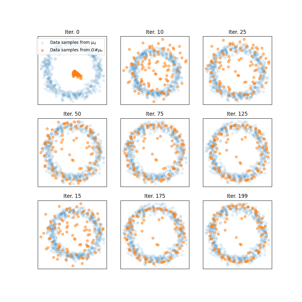
Plot trajectories of generated samples along iterations
pl.figure(3, (10, 10))
ivisu = [0, 10, 25, 50, 75, 125, 15, 175, 199]
for i in range(9):
pl.subplot(3, 3, i + 1)
pl.scatter(xd[:, 0], xd[:, 1], label="Data samples from $\mu_d$", alpha=0.1)
pl.scatter(
xvisu[ivisu[i], :, 0],
xvisu[ivisu[i], :, 1],
label="Data samples from $G\#\mu_n$",
alpha=0.5,
)
pl.xticks(())
pl.yticks(())
pl.title("Iter. {}".format(ivisu[i]))
if i == 0:
pl.legend()
/home/circleci/project/examples/backends/plot_wass2_gan_torch.py:180: SyntaxWarning: invalid escape sequence '\m'
pl.scatter(xd[:, 0], xd[:, 1], label="Data samples from $\mu_d$", alpha=0.1)
/home/circleci/project/examples/backends/plot_wass2_gan_torch.py:184: SyntaxWarning: invalid escape sequence '\#'
label="Data samples from $G\#\mu_n$",
Animate trajectories of generated samples along iteration
pl.figure(4, (8, 8))
def _update_plot(i):
pl.clf()
pl.scatter(xd[:, 0], xd[:, 1], label="Data samples from $\mu_d$", alpha=0.1)
pl.scatter(
xvisu[i, :, 0], xvisu[i, :, 1], label="Data samples from $G\#\mu_n$", alpha=0.5
)
pl.xticks(())
pl.yticks(())
pl.xlim((-1.5, 1.5))
pl.ylim((-1.5, 1.5))
pl.title("Iter. {}".format(i))
return 1
i = 0
pl.scatter(xd[:, 0], xd[:, 1], label="Data samples from $\mu_d$", alpha=0.1)
pl.scatter(
xvisu[i, :, 0], xvisu[i, :, 1], label="Data samples from $G\#\mu_n$", alpha=0.5
)
pl.xticks(())
pl.yticks(())
pl.xlim((-1.5, 1.5))
pl.ylim((-1.5, 1.5))
pl.title("Iter. {}".format(ivisu[i]))
ani = animation.FuncAnimation(
pl.gcf(), _update_plot, n_iter, interval=100, repeat_delay=2000
)