ot.da
Domain adaptation with optimal transport
Functions
- ot.da.distribution_estimation_uniform(X)[source]
estimates a uniform distribution from an array of samples \(\mathbf{X}\)
- Parameters:
X (array-like, shape (n_samples, n_features)) – The array of samples
- Returns:
mu – The uniform distribution estimated from \(\mathbf{X}\)
- Return type:
array-like, shape (n_samples,)
- ot.da.emd_laplace(a, b, xs, xt, M, sim='knn', sim_param=None, reg='pos', eta=1, alpha=0.5, numItermax=100, stopThr=1e-09, numInnerItermax=100000, stopInnerThr=1e-09, log=False, verbose=False)[source]
Solve the optimal transport problem (OT) with Laplacian regularization
\[ \begin{align}\begin{aligned}\gamma = \mathop{\arg \min}_\gamma \quad \langle \gamma, \mathbf{M} \rangle_F + \eta \cdot \Omega_\alpha(\gamma)\\s.t. \ \gamma \mathbf{1} = \mathbf{a}\\ \gamma^T \mathbf{1} = \mathbf{b}\\ \gamma \geq 0\end{aligned}\end{align} \]where:
\(\mathbf{a}\) and \(\mathbf{b}\) are source and target weights (sum to 1)
\(\mathbf{x_s}\) and \(\mathbf{x_t}\) are source and target samples
\(\mathbf{M}\) is the (ns, nt) metric cost matrix
\(\Omega_\alpha\) is the Laplacian regularization term
\[\Omega_\alpha = \frac{1 - \alpha}{n_s^2} \sum_{i,j} \mathbf{S^s}_{i,j} \|T(\mathbf{x}^s_i) - T(\mathbf{x}^s_j) \|^2 + \frac{\alpha}{n_t^2} \sum_{i,j} \mathbf{S^t}_{i,j} \|T(\mathbf{x}^t_i) - T(\mathbf{x}^t_j) \|^2\]with \(\mathbf{S^s}_{i,j}, \mathbf{S^t}_{i,j}\) denoting source and target similarity matrices and \(T(\cdot)\) being a barycentric mapping.
The algorithm used for solving the problem is the conditional gradient algorithm as proposed in [5].
- Parameters:
a (array-like (ns,)) – samples weights in the source domain
b (array-like (nt,)) – samples weights in the target domain
xs (array-like (ns,d)) – samples in the source domain
xt (array-like (nt,d)) – samples in the target domain
M (array-like (ns,nt)) – loss matrix
sim (string, optional) – Type of similarity (‘knn’ or ‘gauss’) used to construct the Laplacian.
sim_param (int or float, optional) – Parameter (number of the nearest neighbors for sim=’knn’ or bandwidth for sim=’gauss’) used to compute the Laplacian.
reg (string) – Type of Laplacian regularization
eta (float) – Regularization term for Laplacian regularization
alpha (float) – Regularization term for source domain’s importance in regularization
numItermax (int, optional) – Max number of iterations
stopThr (float, optional) – Stop threshold on error (inner emd solver) (>0)
numInnerItermax (int, optional) – Max number of iterations (inner CG solver)
stopInnerThr (float, optional) – Stop threshold on error (inner CG solver) (>0)
verbose (bool, optional) – Print information along iterations
log (bool, optional) – record log if True
- Returns:
gamma ((ns, nt) array-like) – Optimal transportation matrix for the given parameters
log (dict) – log dictionary return only if log==True in parameters
References
See also
ot.lp.emdUnregularized OT
ot.optim.cgGeneral regularized OT
- ot.da.sinkhorn_l1l2_gl(a, labels_a, b, M, reg, eta=0.1, numItermax=10, numInnerItermax=200, stopInnerThr=1e-09, eps=1e-12, verbose=False, log=False)[source]
Solve the entropic regularization optimal transport problem with group lasso regularization
The function solves the following optimization problem:
\[ \begin{align}\begin{aligned}\gamma = \mathop{\arg \min}_\gamma \quad \langle \gamma, \mathbf{M} \rangle_F + \mathrm{reg} \cdot \Omega_e(\gamma) + \eta \ \Omega_g(\gamma)\\s.t. \ \gamma \mathbf{1} = \mathbf{a}\\ \gamma^T \mathbf{1} = \mathbf{b}\\ \gamma \geq 0\end{aligned}\end{align} \]where :
\(\mathbf{M}\) is the (ns, nt) metric cost matrix
\(\Omega_e\) is the entropic regularization term \(\Omega_e(\gamma)=\sum_{i,j} \gamma_{i,j}\log(\gamma_{i,j})\)
\(\Omega_g\) is the group lasso regularization term \(\Omega_g(\gamma)=\sum_{i,c} \|\gamma_{i,\mathcal{I}_c}\|^2\) where \(\mathcal{I}_c\) are the index of samples from class c in the source domain.
\(\mathbf{a}\) and \(\mathbf{b}\) are source and target weights (sum to 1)
The algorithm used for solving the problem is the generalized conditional gradient as proposed in [5, 7].
- Parameters:
a (array-like (ns,)) – samples weights in the source domain
labels_a (array-like (ns,)) – labels of samples in the source domain
b (array-like (nt,)) – samples in the target domain
M (array-like (ns,nt)) – loss matrix
reg (float) – Regularization term for entropic regularization >0
eta (float, optional) – Regularization term for group lasso regularization >0
numItermax (int, optional) – Max number of iterations
numInnerItermax (int, optional) – Max number of iterations (inner sinkhorn solver)
stopInnerThr (float, optional) – Stop threshold on error (inner sinkhorn solver) (>0)
eps (float, optional (default=1e-12)) – Small value to avoid division by zero
verbose (bool, optional) – Print information along iterations
log (bool, optional) – record log if True
- Returns:
gamma ((ns, nt) array-like) – Optimal transportation matrix for the given parameters
log (dict) – log dictionary return only if log==True in parameters
References
See also
ot.optim.gcgGeneralized conditional gradient for OT problems
- ot.da.sinkhorn_lpl1_mm(a, labels_a, b, M, reg, eta=0.1, numItermax=10, numInnerItermax=200, stopInnerThr=1e-09, verbose=False, log=False)[source]
Solve the entropic regularization optimal transport problem with non-convex group lasso regularization
The function solves the following optimization problem:
\[ \begin{align}\begin{aligned}\gamma = \mathop{\arg \min}_\gamma \quad \langle \gamma, \mathbf{M} \rangle_F + \mathrm{reg} \cdot \Omega_e(\gamma) + \eta \ \Omega_g(\gamma)\\s.t. \ \gamma \mathbf{1} = \mathbf{a}\\ \gamma^T \mathbf{1} = \mathbf{b}\\ \gamma \geq 0\end{aligned}\end{align} \]where :
\(\mathbf{M}\) is the (ns, nt) metric cost matrix
\(\Omega_e\) is the entropic regularization term \(\Omega_e (\gamma)=\sum_{i,j} \gamma_{i,j}\log(\gamma_{i,j})\)
\(\Omega_g\) is the group lasso regularization term \(\Omega_g(\gamma)=\sum_{i,c} \|\gamma_{i,\mathcal{I}_c}\|^{1/2}_1\) where \(\mathcal{I}_c\) are the index of samples from class c in the source domain.
\(\mathbf{a}\) and \(\mathbf{b}\) are source and target weights (sum to 1)
The algorithm used for solving the problem is the generalized conditional gradient as proposed in [5, 7].
- Parameters:
a (array-like (ns,)) – samples weights in the source domain
labels_a (array-like (ns,)) – labels of samples in the source domain
b (array-like (nt,)) – samples weights in the target domain
M (array-like (ns,nt)) – loss matrix
reg (float) – Regularization term for entropic regularization >0
eta (float, optional) – Regularization term for group lasso regularization >0
numItermax (int, optional) – Max number of iterations
numInnerItermax (int, optional) – Max number of iterations (inner sinkhorn solver)
stopInnerThr (float, optional) – Stop threshold on error (inner sinkhorn solver) (>0)
verbose (bool, optional) – Print information along iterations
log (bool, optional) – record log if True
- Returns:
gamma ((ns, nt) array-like) – Optimal transportation matrix for the given parameters
log (dict) – log dictionary return only if log==True in parameters
References
See also
ot.lp.emdUnregularized OT
ot.bregman.sinkhornEntropic regularized OT
ot.optim.cgGeneral regularized OT
Classes
- class ot.da.BaseTransport[source]
Base class for OTDA objects
Note
All estimators should specify all the parameters that can be set at the class level in their
__init__as explicit keyword arguments (no*argsor**kwargs).The fit method should:
estimate a cost matrix and store it in a cost_ attribute
estimate a coupling matrix and store it in a coupling_ attribute
estimate distributions from source and target data and store them in mu_s and mu_t attributes
store Xs and Xt in attributes to be used later on in transform and inverse_transform methods
transform method should always get as input a Xs parameter
inverse_transform method should always get as input a Xt parameter
transform_labels method should always get as input a ys parameter
inverse_transform_labels method should always get as input a yt parameter
- fit(Xs=None, ys=None, Xt=None, yt=None)[source]
Build a coupling matrix from source and target sets of samples \((\mathbf{X_s}, \mathbf{y_s})\) and \((\mathbf{X_t}, \mathbf{y_t})\)
- Parameters:
Xs (array-like, shape (n_source_samples, n_features)) – The training input samples.
ys (array-like, shape (n_source_samples,)) – The training class labels
Xt (array-like, shape (n_target_samples, n_features)) – The training input samples.
yt (array-like, shape (n_target_samples,)) –
The class labels. If some target samples are unlabelled, fill the \(\mathbf{y_t}\)’s elements with -1.
Warning: Note that, due to this convention -1 cannot be used as a class label
- Returns:
self – Returns self.
- Return type:
- fit_transform(Xs=None, ys=None, Xt=None, yt=None)[source]
Build a coupling matrix from source and target sets of samples \((\mathbf{X_s}, \mathbf{y_s})\) and \((\mathbf{X_t}, \mathbf{y_t})\) and transports source samples \(\mathbf{X_s}\) onto target ones \(\mathbf{X_t}\)
- Parameters:
Xs (array-like, shape (n_source_samples, n_features)) – The training input samples.
ys (array-like, shape (n_source_samples,)) – The class labels for training samples
Xt (array-like, shape (n_target_samples, n_features)) – The training input samples.
yt (array-like, shape (n_target_samples,)) –
The class labels. If some target samples are unlabelled, fill the \(\mathbf{y_t}\)’s elements with -1.
Warning: Note that, due to this convention -1 cannot be used as a class label
- Returns:
transp_Xs – The source samples samples.
- Return type:
array-like, shape (n_source_samples, n_features)
- inverse_transform(Xs=None, ys=None, Xt=None, yt=None, batch_size=128)[source]
Transports target samples \(\mathbf{X_t}\) onto source samples \(\mathbf{X_s}\)
- Parameters:
Xs (array-like, shape (n_source_samples, n_features)) – The source input samples.
ys (array-like, shape (n_source_samples,)) – The source class labels
Xt (array-like, shape (n_target_samples, n_features)) – The target input samples.
yt (array-like, shape (n_target_samples,)) –
The target class labels. If some target samples are unlabelled, fill the \(\mathbf{y_t}\)’s elements with -1.
Warning: Note that, due to this convention -1 cannot be used as a class label
batch_size (int, optional (default=128)) – The batch size for out of sample inverse transform
- Returns:
transp_Xt – The transported target samples.
- Return type:
array-like, shape (n_source_samples, n_features)
- inverse_transform_labels(yt=None)[source]
Propagate target labels \(\mathbf{y_t}\) to obtain estimated source labels \(\mathbf{y_s}\)
- Parameters:
yt (array-like, shape (n_target_samples,))
- Returns:
transp_ys – Estimated soft source labels.
- Return type:
array-like, shape (n_source_samples, nb_classes)
- transform(Xs=None, ys=None, Xt=None, yt=None, batch_size=128)[source]
Transports source samples \(\mathbf{X_s}\) onto target ones \(\mathbf{X_t}\)
- Parameters:
Xs (array-like, shape (n_source_samples, n_features)) – The source input samples.
ys (array-like, shape (n_source_samples,)) – The class labels for source samples
Xt (array-like, shape (n_target_samples, n_features)) – The target input samples.
yt (array-like, shape (n_target_samples,)) –
The class labels for target. If some target samples are unlabelled, fill the \(\mathbf{y_t}\)’s elements with -1.
Warning: Note that, due to this convention -1 cannot be used as a class label
batch_size (int, optional (default=128)) – The batch size for out of sample inverse transform
- Returns:
transp_Xs – The transport source samples.
- Return type:
array-like, shape (n_source_samples, n_features)
- transform_labels(ys=None)[source]
Propagate source labels \(\mathbf{y_s}\) to obtain estimated target labels as in [27].
- Parameters:
ys (array-like, shape (n_source_samples,)) – The source class labels
- Returns:
transp_ys – Estimated soft target labels.
- Return type:
array-like, shape (n_target_samples, nb_classes)
References
Examples using ot.da.BaseTransport
OT with Laplacian regularization for domain adaptation
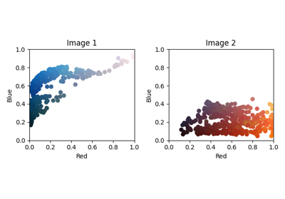
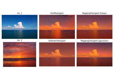
OT for image color adaptation with mapping estimation
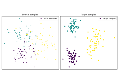
OT for domain adaptation on empirical distributions
- class ot.da.EMDLaplaceTransport(reg_type='pos', reg_lap=1.0, reg_src=1.0, metric='sqeuclidean', norm=None, similarity='knn', similarity_param=None, max_iter=100, tol=1e-09, max_inner_iter=100000, inner_tol=1e-09, log=False, verbose=False, distribution_estimation=<function distribution_estimation_uniform>, out_of_sample_map='ferradans')[source]
Domain Adaptation OT method based on Earth Mover’s Distance with Laplacian regularization
- Parameters:
reg_type (string optional (default='pos')) – Type of the regularization term: ‘pos’ and ‘disp’ for regularization term defined in [2] and [6], respectively.
reg_lap (float, optional (default=1)) – Laplacian regularization parameter
reg_src (float, optional (default=0.5)) – Source relative importance in regularization
metric (string, optional (default="sqeuclidean")) – The ground metric for the Wasserstein problem
norm (string, optional (default=None)) – If given, normalize the ground metric to avoid numerical errors that can occur with large metric values.
similarity (string, optional (default="knn")) – The similarity to use either knn or gaussian
similarity_param (int or float, optional (default=None)) – Parameter for the similarity: number of nearest neighbors or bandwidth if similarity=”knn” or “gaussian”, respectively. If None is provided, it is set to 3 or the average pairwise squared Euclidean distance, respectively.
max_iter (int, optional (default=100)) – Max number of BCD iterations
tol (float, optional (default=1e-5)) – Stop threshold on relative loss decrease (>0)
max_inner_iter (int, optional (default=10)) – Max number of iterations (inner CG solver)
inner_tol (float, optional (default=1e-6)) – Stop threshold on error (inner CG solver) (>0)
log (int, optional (default=False)) – Controls the logs of the optimization algorithm
distribution_estimation (callable, optional (defaults to the uniform)) – The kind of distribution estimation to employ
out_of_sample_map (string, optional (default="ferradans")) – The kind of out of sample mapping to apply to transport samples from a domain into another one. Currently the only possible option is “ferradans” which uses the method proposed in [6].
- coupling_
The optimal coupling
- Type:
array-like, shape (n_source_samples, n_target_samples)
References
- fit(Xs, ys=None, Xt=None, yt=None)[source]
Build a coupling matrix from source and target sets of samples \((\mathbf{X_s}, \mathbf{y_s})\) and \((\mathbf{X_t}, \mathbf{y_t})\)
- Parameters:
Xs (array-like, shape (n_source_samples, n_features)) – The training input samples.
ys (array-like, shape (n_source_samples,)) – The class labels
Xt (array-like, shape (n_target_samples, n_features)) – The training input samples.
yt (array-like, shape (n_target_samples,)) –
The class labels. If some target samples are unlabelled, fill the \(\mathbf{y_t}\)’s elements with -1.
Warning: Note that, due to this convention -1 cannot be used as a class label
- Returns:
self – Returns self.
- Return type:
Examples using ot.da.EMDLaplaceTransport
OT with Laplacian regularization for domain adaptation
- class ot.da.EMDTransport(metric='sqeuclidean', norm=None, log=False, distribution_estimation=<function distribution_estimation_uniform>, out_of_sample_map='ferradans', limit_max=10, max_iter=100000)[source]
Domain Adaptation OT method based on Earth Mover’s Distance
- Parameters:
metric (string, optional (default="sqeuclidean")) – The ground metric for the Wasserstein problem
norm (string, optional (default=None)) – If given, normalize the ground metric to avoid numerical errors that can occur with large metric values.
log (int, optional (default=False)) – Controls the logs of the optimization algorithm
distribution_estimation (callable, optional (defaults to the uniform)) – The kind of distribution estimation to employ
out_of_sample_map (string, optional (default="ferradans")) – The kind of out of sample mapping to apply to transport samples from a domain into another one. Currently the only possible option is “ferradans” which uses the method proposed in [6].
limit_max (float, optional (default=10)) – Controls the semi supervised mode. Transport between labeled source and target samples of different classes will exhibit an infinite cost (10 times the maximum value of the cost matrix)
max_iter (int, optional (default=100000)) – The maximum number of iterations before stopping the optimization algorithm if it has not converged.
- coupling_
The optimal coupling
- Type:
array-like, shape (n_source_samples, n_target_samples)
References
- fit(Xs, ys=None, Xt=None, yt=None)[source]
Build a coupling matrix from source and target sets of samples \((\mathbf{X_s}, \mathbf{y_s})\) and \((\mathbf{X_t}, \mathbf{y_t})\)
- Parameters:
Xs (array-like, shape (n_source_samples, n_features)) – The training input samples.
ys (array-like, shape (n_source_samples,)) – The class labels
Xt (array-like, shape (n_target_samples, n_features)) – The training input samples.
yt (array-like, shape (n_target_samples,)) –
The class labels. If some target samples are unlabelled, fill the \(\mathbf{y_t}\)’s elements with -1.
Warning: Note that, due to this convention -1 cannot be used as a class label
- Returns:
self – Returns self.
- Return type:
Examples using ot.da.EMDTransport
OT with Laplacian regularization for domain adaptation
OT for image color adaptation with mapping estimation
OT for domain adaptation on empirical distributions
- class ot.da.JCPOTTransport(reg_e=0.1, max_iter=10, tol=1e-08, verbose=False, log=False, metric='sqeuclidean', out_of_sample_map='ferradans')[source]
Domain Adaptation OT method for multi-source target shift based on Wasserstein barycenter algorithm.
- Parameters:
reg_e (float, optional (default=1)) – Entropic regularization parameter
max_iter (int, float, optional (default=10)) – The minimum number of iteration before stopping the optimization algorithm if it has not converged
tol (float, optional (default=10e-9)) – Stop threshold on error (inner sinkhorn solver) (>0)
verbose (bool, optional (default=False)) – Controls the verbosity of the optimization algorithm
log (bool, optional (default=False)) – Controls the logs of the optimization algorithm
metric (string, optional (default="sqeuclidean")) – The ground metric for the Wasserstein problem
norm (string, optional (default=None)) – If given, normalize the ground metric to avoid numerical errors that can occur with large metric values.
distribution_estimation (callable, optional (defaults to the uniform)) – The kind of distribution estimation to employ
out_of_sample_map (string, optional (default="ferradans")) – The kind of out of sample mapping to apply to transport samples from a domain into another one. Currently the only possible option is “ferradans” which uses the method proposed in [6].
- coupling_
A set of optimal couplings between each source domain and the target domain
- Type:
list of array-like objects, shape K x (n_source_samples, n_target_samples)
- proportions_
Estimated class proportions in the target domain
- Type:
array-like, shape (n_classes,)
- log_
The dictionary of log, empty dict if parameter log is not True
- Type:
dictionary
References
- fit(Xs, ys=None, Xt=None, yt=None)[source]
Building coupling matrices from a list of source and target sets of samples \((\mathbf{X_s}, \mathbf{y_s})\) and \((\mathbf{X_t}, \mathbf{y_t})\)
- Parameters:
Xs (list of K array-like objects, shape K x (nk_source_samples, n_features)) – A list of the training input samples.
ys (list of K array-like objects, shape K x (nk_source_samples,)) – A list of the class labels
Xt (array-like, shape (n_target_samples, n_features)) – The training input samples.
yt (array-like, shape (n_target_samples,)) –
The class labels. If some target samples are unlabelled, fill the \(\mathbf{y_t}\)’s elements with -1.
Warning: Note that, due to this convention -1 cannot be used as a class label
- Returns:
self – Returns self.
- Return type:
- inverse_transform_labels(yt=None)[source]
Propagate target labels \(\mathbf{y_t}\) to obtain estimated source labels \(\mathbf{y_s}\)
- Parameters:
yt (array-like, shape (n_target_samples,)) – The target class labels
- Returns:
transp_ys – A list of estimated soft source labels
- Return type:
list of K array-like objects, shape K x (nk_source_samples, nb_classes)
- transform(Xs=None, ys=None, Xt=None, yt=None, batch_size=128)[source]
Transports source samples \(\mathbf{X_s}\) onto target ones \(\mathbf{X_t}\)
- Parameters:
Xs (list of K array-like objects, shape K x (nk_source_samples, n_features)) – A list of the training input samples.
ys (list of K array-like objects, shape K x (nk_source_samples,)) – A list of the class labels
Xt (array-like, shape (n_target_samples, n_features)) – The training input samples.
yt (array-like, shape (n_target_samples,)) –
The class labels. If some target samples are unlabelled, fill the \(\mathbf{y_t}\)’s elements with -1.
Warning: Note that, due to this convention -1 cannot be used as a class label
batch_size (int, optional (default=128)) – The batch size for out of sample inverse transform
- transform_labels(ys=None)[source]
Propagate source labels \(\mathbf{y_s}\) to obtain target labels as in [27]
- Parameters:
ys (list of K array-like objects, shape K x (nk_source_samples,)) – A list of the class labels
- Returns:
yt – Estimated soft target labels.
- Return type:
array-like, shape (n_target_samples, nb_classes)
References
Examples using ot.da.JCPOTTransport
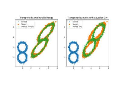
- class ot.da.LinearGWTransport(log=False, sign_eigs=None, distribution_estimation=<function distribution_estimation_uniform>)[source]
OT Gaussian Gromov-Wasserstein linear operator between empirical distributions
The function estimates the optimal linear operator that aligns the two empirical distributions optimally wrt the Gromov-Wasserstein distance. This is equivalent to estimating the closed form mapping between two Gaussian distributions \(\mathcal{N}(\mu_s,\Sigma_s)\) and \(\mathcal{N}(\mu_t,\Sigma_t)\) as proposed in [57].
The linear operator from source to target \(M\)
\[M(\mathbf{x})= \mathbf{A} \mathbf{x} + \mathbf{b}\]where the matrix \(\mathbf{A}\) and the vector \(\mathbf{b}\) are defined in [57].
- Parameters:
sign_eigs (array-like (n_features), str, optional) – sign of the eigenvalues of the mapping matrix, by default all signs will be positive. If ‘skewness’ is provided, the sign of the eigenvalues is selected as the product of the sign of the skewness of the projected data.
log (bool, optional) – record log if True
References
- fit(Xs=None, ys=None, Xt=None, yt=None)[source]
Build a coupling matrix from source and target sets of samples \((\mathbf{X_s}, \mathbf{y_s})\) and \((\mathbf{X_t}, \mathbf{y_t})\)
- Parameters:
Xs (array-like, shape (n_source_samples, n_features)) – The training input samples.
ys (array-like, shape (n_source_samples,)) – The class labels
Xt (array-like, shape (n_target_samples, n_features)) – The training input samples.
yt (array-like, shape (n_target_samples,)) –
The class labels. If some target samples are unlabelled, fill the \(\mathbf{y_t}\)’s elements with -1.
Warning: Note that, due to this convention -1 cannot be used as a class label
- Returns:
self – Returns self.
- Return type:
Examples using ot.da.LinearGWTransport
- class ot.da.LinearTransport(reg=1e-08, bias=True, log=False, distribution_estimation=<function distribution_estimation_uniform>)[source]
OT linear operator between empirical distributions
The function estimates the optimal linear operator that aligns the two empirical distributions. This is equivalent to estimating the closed form mapping between two Gaussian distributions \(\mathcal{N}(\mu_s,\Sigma_s)\) and \(\mathcal{N}(\mu_t,\Sigma_t)\) as proposed in [14] and discussed in remark 2.29 in [15].
The linear operator from source to target \(M\)
\[M(\mathbf{x})= \mathbf{A} \mathbf{x} + \mathbf{b}\]where :
\[ \begin{align}\begin{aligned}\mathbf{A} &= \Sigma_s^{-1/2} \left(\Sigma_s^{1/2}\Sigma_t\Sigma_s^{1/2} \right)^{1/2} \Sigma_s^{-1/2}\\\mathbf{b} &= \mu_t - \mathbf{A} \mu_s\end{aligned}\end{align} \]- Parameters:
References
- fit(Xs=None, ys=None, Xt=None, yt=None)[source]
Build a coupling matrix from source and target sets of samples \((\mathbf{X_s}, \mathbf{y_s})\) and \((\mathbf{X_t}, \mathbf{y_t})\)
- Parameters:
Xs (array-like, shape (n_source_samples, n_features)) – The training input samples.
ys (array-like, shape (n_source_samples,)) – The class labels
Xt (array-like, shape (n_target_samples, n_features)) – The training input samples.
yt (array-like, shape (n_target_samples,)) –
The class labels. If some target samples are unlabelled, fill the \(\mathbf{y_t}\)’s elements with -1.
Warning: Note that, due to this convention -1 cannot be used as a class label
- Returns:
self – Returns self.
- Return type:
- inverse_transform(Xs=None, ys=None, Xt=None, yt=None, batch_size=128)[source]
Transports target samples \(\mathbf{X_t}\) onto source samples \(\mathbf{X_s}\)
- Parameters:
Xs (array-like, shape (n_source_samples, n_features)) – The training input samples.
ys (array-like, shape (n_source_samples,)) – The class labels
Xt (array-like, shape (n_target_samples, n_features)) – The training input samples.
yt (array-like, shape (n_target_samples,)) –
The class labels. If some target samples are unlabelled, fill the \(\mathbf{y_t}\)’s elements with -1.
Warning: Note that, due to this convention -1 cannot be used as a class label
batch_size (int, optional (default=128)) – The batch size for out of sample inverse transform
- Returns:
transp_Xt – The transported target samples.
- Return type:
array-like, shape (n_source_samples, n_features)
- transform(Xs=None, ys=None, Xt=None, yt=None, batch_size=128)[source]
Transports source samples \(\mathbf{X_s}\) onto target ones \(\mathbf{X_t}\)
- Parameters:
Xs (array-like, shape (n_source_samples, n_features)) – The training input samples.
ys (array-like, shape (n_source_samples,)) – The class labels
Xt (array-like, shape (n_target_samples, n_features)) – The training input samples.
yt (array-like, shape (n_target_samples,)) –
The class labels. If some target samples are unlabelled, fill the \(\mathbf{y_t}\)’s elements with -1.
Warning: Note that, due to this convention -1 cannot be used as a class label
batch_size (int, optional (default=128)) – The batch size for out of sample inverse transform
- Returns:
transp_Xs – The transport source samples.
- Return type:
array-like, shape (n_source_samples, n_features)
Examples using ot.da.LinearTransport
- class ot.da.MappingTransport(mu=1, eta=0.001, bias=False, metric='sqeuclidean', norm=None, kernel='linear', sigma=1, max_iter=100, tol=1e-05, max_inner_iter=10, inner_tol=1e-06, log=False, verbose=False, verbose2=False)[source]
MappingTransport: DA methods that aims at jointly estimating a optimal transport coupling and the associated mapping
- Parameters:
mu (float, optional (default=1)) – Weight for the linear OT loss (>0)
eta (float, optional (default=0.001)) – Regularization term for the linear mapping L (>0)
bias (bool, optional (default=False)) – Estimate linear mapping with constant bias
metric (string, optional (default="sqeuclidean")) – The ground metric for the Wasserstein problem
norm (string, optional (default=None)) – If given, normalize the ground metric to avoid numerical errors that can occur with large metric values.
kernel (string, optional (default="linear")) – The kernel to use either linear or gaussian
sigma (float, optional (default=1)) – The gaussian kernel parameter
max_iter (int, optional (default=100)) – Max number of BCD iterations
tol (float, optional (default=1e-5)) – Stop threshold on relative loss decrease (>0)
max_inner_iter (int, optional (default=10)) – Max number of iterations (inner CG solver)
inner_tol (float, optional (default=1e-6)) – Stop threshold on error (inner CG solver) (>0)
log (bool, optional (default=False)) – record log if True
verbose (bool, optional (default=False)) – Print information along iterations
verbose2 (bool, optional (default=False)) – Print information along iterations
- coupling_
The optimal coupling
- Type:
array-like, shape (n_source_samples, n_target_samples)
- mapping_
The associated mapping
array-like, shape (n_features (+ 1), n_features), (if bias) for kernel == linear
array-like, shape (n_source_samples (+ 1), n_features), (if bias) for kernel == gaussian
- log_
The dictionary of log, empty dict if parameter log is not True
- Type:
dictionary
References
- fit(Xs=None, ys=None, Xt=None, yt=None)[source]
Builds an optimal coupling and estimates the associated mapping from source and target sets of samples \((\mathbf{X_s}, \mathbf{y_s})\) and \((\mathbf{X_t}, \mathbf{y_t})\)
- Parameters:
Xs (array-like, shape (n_source_samples, n_features)) – The training input samples.
ys (array-like, shape (n_source_samples,)) – The class labels
Xt (array-like, shape (n_target_samples, n_features)) – The training input samples.
yt (array-like, shape (n_target_samples,)) –
The class labels. If some target samples are unlabelled, fill the \(\mathbf{y_t}\)’s elements with -1.
Warning: Note that, due to this convention -1 cannot be used as a class label
- Returns:
self – Returns self
- Return type:
- transform(Xs)[source]
Transports source samples \(\mathbf{X_s}\) onto target ones \(\mathbf{X_t}\)
- Parameters:
Xs (array-like, shape (n_source_samples, n_features)) – The training input samples.
- Returns:
transp_Xs – The transport source samples.
- Return type:
array-like, shape (n_source_samples, n_features)
Examples using ot.da.MappingTransport
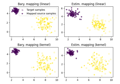
OT for image color adaptation with mapping estimation
- class ot.da.NearestBrenierPotential(strongly_convex_constant=0.6, gradient_lipschitz_constant=1.4, log=False, its=100, seed=None)[source]
Smooth Strongly Convex Nearest Brenier Potentials (SSNB) is a method from [58] that computes an l-strongly convex potential \(\varphi\) with an L-Lipschitz gradient such that \(\nabla \varphi \# \mu \approx \nu\). This regularity can be enforced only on the components of a partition of the ambient space (encoded by point classes), which is a relaxation compared to imposing global regularity.
SSNBs approach the target measure by solving the optimisation problem:
\begin{gather*} \varphi \in \text{argmin}_{\varphi \in \mathcal{F}}\ \text{W}_2(\nabla \varphi \#\mu_s, \mu_t), \end{gather*}where \(\mathcal{F}\) is the space functions that are on every set \(E_k\) l-strongly convex with an L-Lipschitz gradient, given \((E_k)_{k \in [K]}\) a partition of the ambient source space.
The problem is solved on “fitting” source and target data via a convex Quadratically Constrained Quadratic Program, yielding the values
phiand the gradientsGat at the source points. The images of “new” source samples are then found by solving a (simpler) Quadratically Constrained Linear Program at each point, using the fitting “parameters”phiandG. We provide two possible images, which correspond to “lower” and “upper potentials” ([59], Theorem 3.14). Each of these two images are optimal solutions of the SSNB problem, and can be used in practice.Warning
This function requires the CVXPY library
Warning
Accepts any backend but will convert to Numpy then back to the backend.
- Parameters:
strongly_convex_constant (float, optional) – constant for the strong convexity of the input potential phi, defaults to 0.6
gradient_lipschitz_constant (float, optional) – constant for the Lipschitz property of the input gradient G, defaults to 1.4
its (int, optional) – number of iterations, defaults to 100
log (bool, optional) – record log if true
seed (int or RandomState or None, optional) – Seed used for random number generator (for the initialisation in
fit.
References
See also
ot.mapping.nearest_brenier_potential_fitFitting the SSNB on source and target data
ot.mapping.nearest_brenier_potential_predict_boundsPredicting SSNB images on new source data
- fit(Xs=None, ys=None, Xt=None, yt=None)[source]
Fits the Smooth Strongly Convex Nearest Brenier Potential [58] to the source data
Xsto the target dataXt, with the partition given by the (optional) labelsys.Wrapper for
ot.mapping.nearest_brenier_potential_fit.Warning
This function requires the CVXPY library
Warning
Accepts any backend but will convert to Numpy then back to the backend.
- Parameters:
Xs (array-like (n, d)) – source points used to compute the optimal values phi and G
ys (array-like (n,), optional) – classes of the reference points, defaults to a single class
Xt (array-like (n, d)) – values of the gradients at the reference points X
yt (optional) – ignored.
- Returns:
self – Returns self.
- Return type:
References
See also
ot.mapping.nearest_brenier_potential_fitFitting the SSNB on source and target data
- transform(Xs, ys=None)[source]
Computes the images of the new source samples
Xsof classesysby the fitted Smooth Strongly Convex Nearest Brenier Potentials (SSNB) [58]. The output is the images of two SSNB optimal maps, called ‘lower’ and ‘upper’ potentials (from [59], Theorem 3.14).Wrapper for
nearest_brenier_potential_predict_bounds.Warning
This function requires the CVXPY library
Warning
Accepts any backend but will convert to Numpy then back to the backend.
- Parameters:
Xs (array-like (m, d)) – input source points
ys (: array_like (m,), optional) – classes of the input source points, defaults to a single class
- Returns:
G_lu – gradients of the lower and upper bounding potentials at Y (images of the source inputs)
- Return type:
array-like (2, m, d)
References
See also
ot.mapping.nearest_brenier_potential_predict_boundsPredicting SSNB images on new source data
- class ot.da.SinkhornL1l2Transport(reg_e=1.0, reg_cl=0.1, max_iter=10, max_inner_iter=200, tol=1e-08, verbose=False, log=False, metric='sqeuclidean', norm=None, distribution_estimation=<function distribution_estimation_uniform>, out_of_sample_map='ferradans', limit_max=10)[source]
Domain Adaptation OT method based on sinkhorn algorithm + L1L2 class regularization.
- Parameters:
reg_e (float, optional (default=1)) – Entropic regularization parameter
reg_cl (float, optional (default=0.1)) – Class regularization parameter
max_iter (int, float, optional (default=10)) – The minimum number of iteration before stopping the optimization algorithm if it has not converged
max_inner_iter (int, float, optional (default=200)) – The number of iteration in the inner loop
tol (float, optional (default=10e-9)) – Stop threshold on error (inner sinkhorn solver) (>0)
verbose (bool, optional (default=False)) – Controls the verbosity of the optimization algorithm
log (bool, optional (default=False)) – Controls the logs of the optimization algorithm
metric (string, optional (default="sqeuclidean")) – The ground metric for the Wasserstein problem
norm (string, optional (default=None)) – If given, normalize the ground metric to avoid numerical errors that can occur with large metric values.
distribution_estimation (callable, optional (defaults to the uniform)) – The kind of distribution estimation to employ
out_of_sample_map (string, optional (default="ferradans")) – The kind of out of sample mapping to apply to transport samples from a domain into another one. Currently the only possible option is “ferradans” which uses the method proposed in [6].
limit_max (float, optional (default=10)) – Controls the semi supervised mode. Transport between labeled source and target samples of different classes will exhibit an infinite cost (10 times the maximum value of the cost matrix)
- coupling_
The optimal coupling
- Type:
array-like, shape (n_source_samples, n_target_samples)
- log_
The dictionary of log, empty dict if parameter log is not True
- Type:
dictionary
References
- fit(Xs, ys=None, Xt=None, yt=None)[source]
Build a coupling matrix from source and target sets of samples \((\mathbf{X_s}, \mathbf{y_s})\) and \((\mathbf{X_t}, \mathbf{y_t})\)
- Parameters:
Xs (array-like, shape (n_source_samples, n_features)) – The training input samples.
ys (array-like, shape (n_source_samples,)) – The class labels
Xt (array-like, shape (n_target_samples, n_features)) – The training input samples.
yt (array-like, shape (n_target_samples,)) –
The class labels. If some target samples are unlabelled, fill the \(\mathbf{y_t}\)’s elements with -1.
Warning: Note that, due to this convention -1 cannot be used as a class label
- Returns:
self – Returns self.
- Return type:
Examples using ot.da.SinkhornL1l2Transport
- class ot.da.SinkhornLpl1Transport(reg_e=1.0, reg_cl=0.1, max_iter=10, max_inner_iter=200, log=False, tol=1e-08, verbose=False, metric='sqeuclidean', norm=None, distribution_estimation=<function distribution_estimation_uniform>, out_of_sample_map='ferradans', limit_max=inf)[source]
Domain Adaptation OT method based on sinkhorn algorithm + LpL1 class regularization.
- Parameters:
reg_e (float, optional (default=1)) – Entropic regularization parameter
reg_cl (float, optional (default=0.1)) – Class regularization parameter
max_iter (int, float, optional (default=10)) – The minimum number of iteration before stopping the optimization algorithm if it has not converged
max_inner_iter (int, float, optional (default=200)) – The number of iteration in the inner loop
log (bool, optional (default=False)) – Controls the logs of the optimization algorithm
tol (float, optional (default=10e-9)) – Stop threshold on error (inner sinkhorn solver) (>0)
verbose (bool, optional (default=False)) – Controls the verbosity of the optimization algorithm
metric (string, optional (default="sqeuclidean")) – The ground metric for the Wasserstein problem
norm (string, optional (default=None)) – If given, normalize the ground metric to avoid numerical errors that can occur with large metric values.
distribution_estimation (callable, optional (defaults to the uniform)) – The kind of distribution estimation to employ
out_of_sample_map (string, optional (default="ferradans")) – The kind of out of sample mapping to apply to transport samples from a domain into another one. Currently the only possible option is “ferradans” which uses the method proposed in [6].
limit_max (float, optional (default=np.inf)) – Controls the semi supervised mode. Transport between labeled source and target samples of different classes will exhibit a cost defined by limit_max.
- coupling_
The optimal coupling
- Type:
array-like, shape (n_source_samples, n_target_samples)
References
- fit(Xs, ys=None, Xt=None, yt=None)[source]
Build a coupling matrix from source and target sets of samples \((\mathbf{X_s}, \mathbf{y_s})\) and \((\mathbf{X_t}, \mathbf{y_t})\)
- Parameters:
Xs (array-like, shape (n_source_samples, n_features)) – The training input samples.
ys (array-like, shape (n_source_samples,)) – The class labels
Xt (array-like, shape (n_target_samples, n_features)) – The training input samples.
yt (array-like, shape (n_target_samples,)) –
The class labels. If some target samples are unlabelled, fill the \(\mathbf{y_t}\)’s elements with -1.
Warning: Note that, due to this convention -1 cannot be used as a class label
- Returns:
self – Returns self.
- Return type:
Examples using ot.da.SinkhornLpl1Transport
OT for domain adaptation on empirical distributions
- class ot.da.SinkhornTransport(reg_e=1.0, method='sinkhorn_log', max_iter=1000, tol=1e-08, verbose=False, log=False, metric='sqeuclidean', norm=None, distribution_estimation=<function distribution_estimation_uniform>, out_of_sample_map='continuous', limit_max=inf)[source]
Domain Adaptation OT method based on Sinkhorn Algorithm
- Parameters:
reg_e (float, optional (default=1)) – Entropic regularization parameter
max_iter (int, float, optional (default=1000)) – The minimum number of iteration before stopping the optimization algorithm if it has not converged
tol (float, optional (default=10e-9)) – The precision required to stop the optimization algorithm.
verbose (bool, optional (default=False)) – Controls the verbosity of the optimization algorithm
log (int, optional (default=False)) – Controls the logs of the optimization algorithm
metric (string, optional (default="sqeuclidean")) – The ground metric for the Wasserstein problem
norm (string, optional (default=None)) – If given, normalize the ground metric to avoid numerical errors that can occur with large metric values. Accepted values are ‘median’, ‘max’, ‘log’ and ‘loglog’.
distribution_estimation (callable, optional (defaults to the uniform)) – The kind of distribution estimation to employ
out_of_sample_map (string, optional (default="continuous")) – The kind of out of sample mapping to apply to transport samples from a domain into another one. Currently the only possible option is “ferradans” which uses the nearest neighbor method proposed in [6] while “continuous” use the out of sample method from [66] and [19].
limit_max (float, optional (default=np.inf)) – Controls the semi supervised mode. Transport between labeled source and target samples of different classes will exhibit an cost defined by this variable
- coupling_
The optimal coupling
- Type:
array-like, shape (n_source_samples, n_target_samples)
- log_
The dictionary of log, empty dict if parameter log is not True
- Type:
dictionary
References
- fit(Xs=None, ys=None, Xt=None, yt=None)[source]
Build a coupling matrix from source and target sets of samples \((\mathbf{X_s}, \mathbf{y_s})\) and \((\mathbf{X_t}, \mathbf{y_t})\)
- Parameters:
Xs (array-like, shape (n_source_samples, n_features)) – The training input samples.
ys (array-like, shape (n_source_samples,)) – The class labels
Xt (array-like, shape (n_target_samples, n_features)) – The training input samples.
yt (array-like, shape (n_target_samples,)) –
The class labels. If some target samples are unlabelled, fill the \(\mathbf{y_t}\)’s elements with -1.
Warning: Note that, due to this convention -1 cannot be used as a class label
- Returns:
self – Returns self.
- Return type:
- inverse_transform(Xs=None, ys=None, Xt=None, yt=None, batch_size=128)[source]
Transports target samples \(\mathbf{X_t}\) onto source samples \(\mathbf{X_s}\)
- Parameters:
Xs (array-like, shape (n_source_samples, n_features)) – The source input samples.
ys (array-like, shape (n_source_samples,)) – The class labels for source samples
Xt (array-like, shape (n_target_samples, n_features)) – The target input samples.
yt (array-like, shape (n_target_samples,)) –
The class labels for target. If some target samples are unlabelled, fill the \(\mathbf{y_t}\)’s elements with -1.
Warning: Note that, due to this convention -1 cannot be used as a class label
batch_size (int, optional (default=128)) – The batch size for out of sample inverse transform
- Returns:
transp_Xt – The transport target samples.
- Return type:
array-like, shape (n_source_samples, n_features)
- transform(Xs=None, ys=None, Xt=None, yt=None, batch_size=128)[source]
Transports source samples \(\mathbf{X_s}\) onto target ones \(\mathbf{X_t}\)
- Parameters:
Xs (array-like, shape (n_source_samples, n_features)) – The source input samples.
ys (array-like, shape (n_source_samples,)) – The class labels for source samples
Xt (array-like, shape (n_target_samples, n_features)) – The target input samples.
yt (array-like, shape (n_target_samples,)) –
The class labels for target. If some target samples are unlabelled, fill the \(\mathbf{y_t}\)’s elements with -1.
Warning: Note that, due to this convention -1 cannot be used as a class label
batch_size (int, optional (default=128)) – The batch size for out of sample inverse transform
- Returns:
transp_Xs – The transport source samples.
- Return type:
array-like, shape (n_source_samples, n_features)
Examples using ot.da.SinkhornTransport
OT with Laplacian regularization for domain adaptation
OT for image color adaptation with mapping estimation
OT for domain adaptation on empirical distributions
- class ot.da.UnbalancedSinkhornTransport(reg_e=1.0, reg_m=0.1, method='sinkhorn', max_iter=10, tol=1e-09, verbose=False, log=False, metric='sqeuclidean', norm=None, distribution_estimation=<function distribution_estimation_uniform>, out_of_sample_map='ferradans', limit_max=10)[source]
Domain Adaptation unbalanced OT method based on sinkhorn algorithm
- Parameters:
reg_e (float, optional (default=1)) – Entropic regularization parameter
reg_m (float, optional (default=0.1)) – Mass regularization parameter
method (str) – method used for the solver either ‘sinkhorn’, ‘sinkhorn_stabilized’ or ‘sinkhorn_epsilon_scaling’, see those function for specific parameters
max_iter (int, float, optional (default=10)) – The minimum number of iteration before stopping the optimization algorithm if it has not converged
tol (float, optional (default=10e-9)) – Stop threshold on error (inner sinkhorn solver) (>0)
verbose (bool, optional (default=False)) – Controls the verbosity of the optimization algorithm
log (bool, optional (default=False)) – Controls the logs of the optimization algorithm
metric (string, optional (default="sqeuclidean")) – The ground metric for the Wasserstein problem
norm (string, optional (default=None)) – If given, normalize the ground metric to avoid numerical errors that can occur with large metric values.
distribution_estimation (callable, optional (defaults to the uniform)) – The kind of distribution estimation to employ
out_of_sample_map (string, optional (default="ferradans")) – The kind of out of sample mapping to apply to transport samples from a domain into another one. Currently the only possible option is “ferradans” which uses the method proposed in [6].
limit_max (float, optional (default=10)) – Controls the semi supervised mode. Transport between labeled source and target samples of different classes will exhibit an infinite cost (10 times the maximum value of the cost matrix)
- coupling_
The optimal coupling
- Type:
array-like, shape (n_source_samples, n_target_samples)
- log_
The dictionary of log, empty dict if parameter log is not True
- Type:
dictionary
References
- fit(Xs, ys=None, Xt=None, yt=None)[source]
Build a coupling matrix from source and target sets of samples \((\mathbf{X_s}, \mathbf{y_s})\) and \((\mathbf{X_t}, \mathbf{y_t})\)
- Parameters:
Xs (array-like, shape (n_source_samples, n_features)) – The training input samples.
ys (array-like, shape (n_source_samples,)) – The class labels
Xt (array-like, shape (n_target_samples, n_features)) – The training input samples.
yt (array-like, shape (n_target_samples,)) –
The class labels. If some target samples are unlabelled, fill the \(\mathbf{y_t}\)’s elements with -1.
Warning: Note that, due to this convention -1 cannot be used as a class label
- Returns:
self – Returns self.
- Return type:
- class ot.da.BaseTransport[source]
Base class for OTDA objects
Note
All estimators should specify all the parameters that can be set at the class level in their
__init__as explicit keyword arguments (no*argsor**kwargs).The fit method should:
estimate a cost matrix and store it in a cost_ attribute
estimate a coupling matrix and store it in a coupling_ attribute
estimate distributions from source and target data and store them in mu_s and mu_t attributes
store Xs and Xt in attributes to be used later on in transform and inverse_transform methods
transform method should always get as input a Xs parameter
inverse_transform method should always get as input a Xt parameter
transform_labels method should always get as input a ys parameter
inverse_transform_labels method should always get as input a yt parameter
- fit(Xs=None, ys=None, Xt=None, yt=None)[source]
Build a coupling matrix from source and target sets of samples \((\mathbf{X_s}, \mathbf{y_s})\) and \((\mathbf{X_t}, \mathbf{y_t})\)
- Parameters:
Xs (array-like, shape (n_source_samples, n_features)) – The training input samples.
ys (array-like, shape (n_source_samples,)) – The training class labels
Xt (array-like, shape (n_target_samples, n_features)) – The training input samples.
yt (array-like, shape (n_target_samples,)) –
The class labels. If some target samples are unlabelled, fill the \(\mathbf{y_t}\)’s elements with -1.
Warning: Note that, due to this convention -1 cannot be used as a class label
- Returns:
self – Returns self.
- Return type:
- fit_transform(Xs=None, ys=None, Xt=None, yt=None)[source]
Build a coupling matrix from source and target sets of samples \((\mathbf{X_s}, \mathbf{y_s})\) and \((\mathbf{X_t}, \mathbf{y_t})\) and transports source samples \(\mathbf{X_s}\) onto target ones \(\mathbf{X_t}\)
- Parameters:
Xs (array-like, shape (n_source_samples, n_features)) – The training input samples.
ys (array-like, shape (n_source_samples,)) – The class labels for training samples
Xt (array-like, shape (n_target_samples, n_features)) – The training input samples.
yt (array-like, shape (n_target_samples,)) –
The class labels. If some target samples are unlabelled, fill the \(\mathbf{y_t}\)’s elements with -1.
Warning: Note that, due to this convention -1 cannot be used as a class label
- Returns:
transp_Xs – The source samples samples.
- Return type:
array-like, shape (n_source_samples, n_features)
- inverse_transform(Xs=None, ys=None, Xt=None, yt=None, batch_size=128)[source]
Transports target samples \(\mathbf{X_t}\) onto source samples \(\mathbf{X_s}\)
- Parameters:
Xs (array-like, shape (n_source_samples, n_features)) – The source input samples.
ys (array-like, shape (n_source_samples,)) – The source class labels
Xt (array-like, shape (n_target_samples, n_features)) – The target input samples.
yt (array-like, shape (n_target_samples,)) –
The target class labels. If some target samples are unlabelled, fill the \(\mathbf{y_t}\)’s elements with -1.
Warning: Note that, due to this convention -1 cannot be used as a class label
batch_size (int, optional (default=128)) – The batch size for out of sample inverse transform
- Returns:
transp_Xt – The transported target samples.
- Return type:
array-like, shape (n_source_samples, n_features)
- inverse_transform_labels(yt=None)[source]
Propagate target labels \(\mathbf{y_t}\) to obtain estimated source labels \(\mathbf{y_s}\)
- Parameters:
yt (array-like, shape (n_target_samples,))
- Returns:
transp_ys – Estimated soft source labels.
- Return type:
array-like, shape (n_source_samples, nb_classes)
- transform(Xs=None, ys=None, Xt=None, yt=None, batch_size=128)[source]
Transports source samples \(\mathbf{X_s}\) onto target ones \(\mathbf{X_t}\)
- Parameters:
Xs (array-like, shape (n_source_samples, n_features)) – The source input samples.
ys (array-like, shape (n_source_samples,)) – The class labels for source samples
Xt (array-like, shape (n_target_samples, n_features)) – The target input samples.
yt (array-like, shape (n_target_samples,)) –
The class labels for target. If some target samples are unlabelled, fill the \(\mathbf{y_t}\)’s elements with -1.
Warning: Note that, due to this convention -1 cannot be used as a class label
batch_size (int, optional (default=128)) – The batch size for out of sample inverse transform
- Returns:
transp_Xs – The transport source samples.
- Return type:
array-like, shape (n_source_samples, n_features)
- transform_labels(ys=None)[source]
Propagate source labels \(\mathbf{y_s}\) to obtain estimated target labels as in [27].
- Parameters:
ys (array-like, shape (n_source_samples,)) – The source class labels
- Returns:
transp_ys – Estimated soft target labels.
- Return type:
array-like, shape (n_target_samples, nb_classes)
References
- class ot.da.EMDLaplaceTransport(reg_type='pos', reg_lap=1.0, reg_src=1.0, metric='sqeuclidean', norm=None, similarity='knn', similarity_param=None, max_iter=100, tol=1e-09, max_inner_iter=100000, inner_tol=1e-09, log=False, verbose=False, distribution_estimation=<function distribution_estimation_uniform>, out_of_sample_map='ferradans')[source]
Domain Adaptation OT method based on Earth Mover’s Distance with Laplacian regularization
- Parameters:
reg_type (string optional (default='pos')) – Type of the regularization term: ‘pos’ and ‘disp’ for regularization term defined in [2] and [6], respectively.
reg_lap (float, optional (default=1)) – Laplacian regularization parameter
reg_src (float, optional (default=0.5)) – Source relative importance in regularization
metric (string, optional (default="sqeuclidean")) – The ground metric for the Wasserstein problem
norm (string, optional (default=None)) – If given, normalize the ground metric to avoid numerical errors that can occur with large metric values.
similarity (string, optional (default="knn")) – The similarity to use either knn or gaussian
similarity_param (int or float, optional (default=None)) – Parameter for the similarity: number of nearest neighbors or bandwidth if similarity=”knn” or “gaussian”, respectively. If None is provided, it is set to 3 or the average pairwise squared Euclidean distance, respectively.
max_iter (int, optional (default=100)) – Max number of BCD iterations
tol (float, optional (default=1e-5)) – Stop threshold on relative loss decrease (>0)
max_inner_iter (int, optional (default=10)) – Max number of iterations (inner CG solver)
inner_tol (float, optional (default=1e-6)) – Stop threshold on error (inner CG solver) (>0)
log (int, optional (default=False)) – Controls the logs of the optimization algorithm
distribution_estimation (callable, optional (defaults to the uniform)) – The kind of distribution estimation to employ
out_of_sample_map (string, optional (default="ferradans")) – The kind of out of sample mapping to apply to transport samples from a domain into another one. Currently the only possible option is “ferradans” which uses the method proposed in [6].
- coupling_
The optimal coupling
- Type:
array-like, shape (n_source_samples, n_target_samples)
References
- fit(Xs, ys=None, Xt=None, yt=None)[source]
Build a coupling matrix from source and target sets of samples \((\mathbf{X_s}, \mathbf{y_s})\) and \((\mathbf{X_t}, \mathbf{y_t})\)
- Parameters:
Xs (array-like, shape (n_source_samples, n_features)) – The training input samples.
ys (array-like, shape (n_source_samples,)) – The class labels
Xt (array-like, shape (n_target_samples, n_features)) – The training input samples.
yt (array-like, shape (n_target_samples,)) –
The class labels. If some target samples are unlabelled, fill the \(\mathbf{y_t}\)’s elements with -1.
Warning: Note that, due to this convention -1 cannot be used as a class label
- Returns:
self – Returns self.
- Return type:
- class ot.da.EMDTransport(metric='sqeuclidean', norm=None, log=False, distribution_estimation=<function distribution_estimation_uniform>, out_of_sample_map='ferradans', limit_max=10, max_iter=100000)[source]
Domain Adaptation OT method based on Earth Mover’s Distance
- Parameters:
metric (string, optional (default="sqeuclidean")) – The ground metric for the Wasserstein problem
norm (string, optional (default=None)) – If given, normalize the ground metric to avoid numerical errors that can occur with large metric values.
log (int, optional (default=False)) – Controls the logs of the optimization algorithm
distribution_estimation (callable, optional (defaults to the uniform)) – The kind of distribution estimation to employ
out_of_sample_map (string, optional (default="ferradans")) – The kind of out of sample mapping to apply to transport samples from a domain into another one. Currently the only possible option is “ferradans” which uses the method proposed in [6].
limit_max (float, optional (default=10)) – Controls the semi supervised mode. Transport between labeled source and target samples of different classes will exhibit an infinite cost (10 times the maximum value of the cost matrix)
max_iter (int, optional (default=100000)) – The maximum number of iterations before stopping the optimization algorithm if it has not converged.
- coupling_
The optimal coupling
- Type:
array-like, shape (n_source_samples, n_target_samples)
References
- fit(Xs, ys=None, Xt=None, yt=None)[source]
Build a coupling matrix from source and target sets of samples \((\mathbf{X_s}, \mathbf{y_s})\) and \((\mathbf{X_t}, \mathbf{y_t})\)
- Parameters:
Xs (array-like, shape (n_source_samples, n_features)) – The training input samples.
ys (array-like, shape (n_source_samples,)) – The class labels
Xt (array-like, shape (n_target_samples, n_features)) – The training input samples.
yt (array-like, shape (n_target_samples,)) –
The class labels. If some target samples are unlabelled, fill the \(\mathbf{y_t}\)’s elements with -1.
Warning: Note that, due to this convention -1 cannot be used as a class label
- Returns:
self – Returns self.
- Return type:
- class ot.da.JCPOTTransport(reg_e=0.1, max_iter=10, tol=1e-08, verbose=False, log=False, metric='sqeuclidean', out_of_sample_map='ferradans')[source]
Domain Adaptation OT method for multi-source target shift based on Wasserstein barycenter algorithm.
- Parameters:
reg_e (float, optional (default=1)) – Entropic regularization parameter
max_iter (int, float, optional (default=10)) – The minimum number of iteration before stopping the optimization algorithm if it has not converged
tol (float, optional (default=10e-9)) – Stop threshold on error (inner sinkhorn solver) (>0)
verbose (bool, optional (default=False)) – Controls the verbosity of the optimization algorithm
log (bool, optional (default=False)) – Controls the logs of the optimization algorithm
metric (string, optional (default="sqeuclidean")) – The ground metric for the Wasserstein problem
norm (string, optional (default=None)) – If given, normalize the ground metric to avoid numerical errors that can occur with large metric values.
distribution_estimation (callable, optional (defaults to the uniform)) – The kind of distribution estimation to employ
out_of_sample_map (string, optional (default="ferradans")) – The kind of out of sample mapping to apply to transport samples from a domain into another one. Currently the only possible option is “ferradans” which uses the method proposed in [6].
- coupling_
A set of optimal couplings between each source domain and the target domain
- Type:
list of array-like objects, shape K x (n_source_samples, n_target_samples)
- proportions_
Estimated class proportions in the target domain
- Type:
array-like, shape (n_classes,)
- log_
The dictionary of log, empty dict if parameter log is not True
- Type:
dictionary
References
- fit(Xs, ys=None, Xt=None, yt=None)[source]
Building coupling matrices from a list of source and target sets of samples \((\mathbf{X_s}, \mathbf{y_s})\) and \((\mathbf{X_t}, \mathbf{y_t})\)
- Parameters:
Xs (list of K array-like objects, shape K x (nk_source_samples, n_features)) – A list of the training input samples.
ys (list of K array-like objects, shape K x (nk_source_samples,)) – A list of the class labels
Xt (array-like, shape (n_target_samples, n_features)) – The training input samples.
yt (array-like, shape (n_target_samples,)) –
The class labels. If some target samples are unlabelled, fill the \(\mathbf{y_t}\)’s elements with -1.
Warning: Note that, due to this convention -1 cannot be used as a class label
- Returns:
self – Returns self.
- Return type:
- inverse_transform_labels(yt=None)[source]
Propagate target labels \(\mathbf{y_t}\) to obtain estimated source labels \(\mathbf{y_s}\)
- Parameters:
yt (array-like, shape (n_target_samples,)) – The target class labels
- Returns:
transp_ys – A list of estimated soft source labels
- Return type:
list of K array-like objects, shape K x (nk_source_samples, nb_classes)
- transform(Xs=None, ys=None, Xt=None, yt=None, batch_size=128)[source]
Transports source samples \(\mathbf{X_s}\) onto target ones \(\mathbf{X_t}\)
- Parameters:
Xs (list of K array-like objects, shape K x (nk_source_samples, n_features)) – A list of the training input samples.
ys (list of K array-like objects, shape K x (nk_source_samples,)) – A list of the class labels
Xt (array-like, shape (n_target_samples, n_features)) – The training input samples.
yt (array-like, shape (n_target_samples,)) –
The class labels. If some target samples are unlabelled, fill the \(\mathbf{y_t}\)’s elements with -1.
Warning: Note that, due to this convention -1 cannot be used as a class label
batch_size (int, optional (default=128)) – The batch size for out of sample inverse transform
- transform_labels(ys=None)[source]
Propagate source labels \(\mathbf{y_s}\) to obtain target labels as in [27]
- Parameters:
ys (list of K array-like objects, shape K x (nk_source_samples,)) – A list of the class labels
- Returns:
yt – Estimated soft target labels.
- Return type:
array-like, shape (n_target_samples, nb_classes)
References
- class ot.da.LinearGWTransport(log=False, sign_eigs=None, distribution_estimation=<function distribution_estimation_uniform>)[source]
OT Gaussian Gromov-Wasserstein linear operator between empirical distributions
The function estimates the optimal linear operator that aligns the two empirical distributions optimally wrt the Gromov-Wasserstein distance. This is equivalent to estimating the closed form mapping between two Gaussian distributions \(\mathcal{N}(\mu_s,\Sigma_s)\) and \(\mathcal{N}(\mu_t,\Sigma_t)\) as proposed in [57].
The linear operator from source to target \(M\)
\[M(\mathbf{x})= \mathbf{A} \mathbf{x} + \mathbf{b}\]where the matrix \(\mathbf{A}\) and the vector \(\mathbf{b}\) are defined in [57].
- Parameters:
sign_eigs (array-like (n_features), str, optional) – sign of the eigenvalues of the mapping matrix, by default all signs will be positive. If ‘skewness’ is provided, the sign of the eigenvalues is selected as the product of the sign of the skewness of the projected data.
log (bool, optional) – record log if True
References
- fit(Xs=None, ys=None, Xt=None, yt=None)[source]
Build a coupling matrix from source and target sets of samples \((\mathbf{X_s}, \mathbf{y_s})\) and \((\mathbf{X_t}, \mathbf{y_t})\)
- Parameters:
Xs (array-like, shape (n_source_samples, n_features)) – The training input samples.
ys (array-like, shape (n_source_samples,)) – The class labels
Xt (array-like, shape (n_target_samples, n_features)) – The training input samples.
yt (array-like, shape (n_target_samples,)) –
The class labels. If some target samples are unlabelled, fill the \(\mathbf{y_t}\)’s elements with -1.
Warning: Note that, due to this convention -1 cannot be used as a class label
- Returns:
self – Returns self.
- Return type:
- class ot.da.LinearTransport(reg=1e-08, bias=True, log=False, distribution_estimation=<function distribution_estimation_uniform>)[source]
OT linear operator between empirical distributions
The function estimates the optimal linear operator that aligns the two empirical distributions. This is equivalent to estimating the closed form mapping between two Gaussian distributions \(\mathcal{N}(\mu_s,\Sigma_s)\) and \(\mathcal{N}(\mu_t,\Sigma_t)\) as proposed in [14] and discussed in remark 2.29 in [15].
The linear operator from source to target \(M\)
\[M(\mathbf{x})= \mathbf{A} \mathbf{x} + \mathbf{b}\]where :
\[ \begin{align}\begin{aligned}\mathbf{A} &= \Sigma_s^{-1/2} \left(\Sigma_s^{1/2}\Sigma_t\Sigma_s^{1/2} \right)^{1/2} \Sigma_s^{-1/2}\\\mathbf{b} &= \mu_t - \mathbf{A} \mu_s\end{aligned}\end{align} \]- Parameters:
References
- fit(Xs=None, ys=None, Xt=None, yt=None)[source]
Build a coupling matrix from source and target sets of samples \((\mathbf{X_s}, \mathbf{y_s})\) and \((\mathbf{X_t}, \mathbf{y_t})\)
- Parameters:
Xs (array-like, shape (n_source_samples, n_features)) – The training input samples.
ys (array-like, shape (n_source_samples,)) – The class labels
Xt (array-like, shape (n_target_samples, n_features)) – The training input samples.
yt (array-like, shape (n_target_samples,)) –
The class labels. If some target samples are unlabelled, fill the \(\mathbf{y_t}\)’s elements with -1.
Warning: Note that, due to this convention -1 cannot be used as a class label
- Returns:
self – Returns self.
- Return type:
- inverse_transform(Xs=None, ys=None, Xt=None, yt=None, batch_size=128)[source]
Transports target samples \(\mathbf{X_t}\) onto source samples \(\mathbf{X_s}\)
- Parameters:
Xs (array-like, shape (n_source_samples, n_features)) – The training input samples.
ys (array-like, shape (n_source_samples,)) – The class labels
Xt (array-like, shape (n_target_samples, n_features)) – The training input samples.
yt (array-like, shape (n_target_samples,)) –
The class labels. If some target samples are unlabelled, fill the \(\mathbf{y_t}\)’s elements with -1.
Warning: Note that, due to this convention -1 cannot be used as a class label
batch_size (int, optional (default=128)) – The batch size for out of sample inverse transform
- Returns:
transp_Xt – The transported target samples.
- Return type:
array-like, shape (n_source_samples, n_features)
- transform(Xs=None, ys=None, Xt=None, yt=None, batch_size=128)[source]
Transports source samples \(\mathbf{X_s}\) onto target ones \(\mathbf{X_t}\)
- Parameters:
Xs (array-like, shape (n_source_samples, n_features)) – The training input samples.
ys (array-like, shape (n_source_samples,)) – The class labels
Xt (array-like, shape (n_target_samples, n_features)) – The training input samples.
yt (array-like, shape (n_target_samples,)) –
The class labels. If some target samples are unlabelled, fill the \(\mathbf{y_t}\)’s elements with -1.
Warning: Note that, due to this convention -1 cannot be used as a class label
batch_size (int, optional (default=128)) – The batch size for out of sample inverse transform
- Returns:
transp_Xs – The transport source samples.
- Return type:
array-like, shape (n_source_samples, n_features)
- class ot.da.MappingTransport(mu=1, eta=0.001, bias=False, metric='sqeuclidean', norm=None, kernel='linear', sigma=1, max_iter=100, tol=1e-05, max_inner_iter=10, inner_tol=1e-06, log=False, verbose=False, verbose2=False)[source]
MappingTransport: DA methods that aims at jointly estimating a optimal transport coupling and the associated mapping
- Parameters:
mu (float, optional (default=1)) – Weight for the linear OT loss (>0)
eta (float, optional (default=0.001)) – Regularization term for the linear mapping L (>0)
bias (bool, optional (default=False)) – Estimate linear mapping with constant bias
metric (string, optional (default="sqeuclidean")) – The ground metric for the Wasserstein problem
norm (string, optional (default=None)) – If given, normalize the ground metric to avoid numerical errors that can occur with large metric values.
kernel (string, optional (default="linear")) – The kernel to use either linear or gaussian
sigma (float, optional (default=1)) – The gaussian kernel parameter
max_iter (int, optional (default=100)) – Max number of BCD iterations
tol (float, optional (default=1e-5)) – Stop threshold on relative loss decrease (>0)
max_inner_iter (int, optional (default=10)) – Max number of iterations (inner CG solver)
inner_tol (float, optional (default=1e-6)) – Stop threshold on error (inner CG solver) (>0)
log (bool, optional (default=False)) – record log if True
verbose (bool, optional (default=False)) – Print information along iterations
verbose2 (bool, optional (default=False)) – Print information along iterations
- coupling_
The optimal coupling
- Type:
array-like, shape (n_source_samples, n_target_samples)
- mapping_
The associated mapping
array-like, shape (n_features (+ 1), n_features), (if bias) for kernel == linear
array-like, shape (n_source_samples (+ 1), n_features), (if bias) for kernel == gaussian
- log_
The dictionary of log, empty dict if parameter log is not True
- Type:
dictionary
References
- fit(Xs=None, ys=None, Xt=None, yt=None)[source]
Builds an optimal coupling and estimates the associated mapping from source and target sets of samples \((\mathbf{X_s}, \mathbf{y_s})\) and \((\mathbf{X_t}, \mathbf{y_t})\)
- Parameters:
Xs (array-like, shape (n_source_samples, n_features)) – The training input samples.
ys (array-like, shape (n_source_samples,)) – The class labels
Xt (array-like, shape (n_target_samples, n_features)) – The training input samples.
yt (array-like, shape (n_target_samples,)) –
The class labels. If some target samples are unlabelled, fill the \(\mathbf{y_t}\)’s elements with -1.
Warning: Note that, due to this convention -1 cannot be used as a class label
- Returns:
self – Returns self
- Return type:
- transform(Xs)[source]
Transports source samples \(\mathbf{X_s}\) onto target ones \(\mathbf{X_t}\)
- Parameters:
Xs (array-like, shape (n_source_samples, n_features)) – The training input samples.
- Returns:
transp_Xs – The transport source samples.
- Return type:
array-like, shape (n_source_samples, n_features)
- class ot.da.NearestBrenierPotential(strongly_convex_constant=0.6, gradient_lipschitz_constant=1.4, log=False, its=100, seed=None)[source]
Smooth Strongly Convex Nearest Brenier Potentials (SSNB) is a method from [58] that computes an l-strongly convex potential \(\varphi\) with an L-Lipschitz gradient such that \(\nabla \varphi \# \mu \approx \nu\). This regularity can be enforced only on the components of a partition of the ambient space (encoded by point classes), which is a relaxation compared to imposing global regularity.
SSNBs approach the target measure by solving the optimisation problem:
\begin{gather*} \varphi \in \text{argmin}_{\varphi \in \mathcal{F}}\ \text{W}_2(\nabla \varphi \#\mu_s, \mu_t), \end{gather*}where \(\mathcal{F}\) is the space functions that are on every set \(E_k\) l-strongly convex with an L-Lipschitz gradient, given \((E_k)_{k \in [K]}\) a partition of the ambient source space.
The problem is solved on “fitting” source and target data via a convex Quadratically Constrained Quadratic Program, yielding the values
phiand the gradientsGat at the source points. The images of “new” source samples are then found by solving a (simpler) Quadratically Constrained Linear Program at each point, using the fitting “parameters”phiandG. We provide two possible images, which correspond to “lower” and “upper potentials” ([59], Theorem 3.14). Each of these two images are optimal solutions of the SSNB problem, and can be used in practice.Warning
This function requires the CVXPY library
Warning
Accepts any backend but will convert to Numpy then back to the backend.
- Parameters:
strongly_convex_constant (float, optional) – constant for the strong convexity of the input potential phi, defaults to 0.6
gradient_lipschitz_constant (float, optional) – constant for the Lipschitz property of the input gradient G, defaults to 1.4
its (int, optional) – number of iterations, defaults to 100
log (bool, optional) – record log if true
seed (int or RandomState or None, optional) – Seed used for random number generator (for the initialisation in
fit.
References
See also
ot.mapping.nearest_brenier_potential_fitFitting the SSNB on source and target data
ot.mapping.nearest_brenier_potential_predict_boundsPredicting SSNB images on new source data
- fit(Xs=None, ys=None, Xt=None, yt=None)[source]
Fits the Smooth Strongly Convex Nearest Brenier Potential [58] to the source data
Xsto the target dataXt, with the partition given by the (optional) labelsys.Wrapper for
ot.mapping.nearest_brenier_potential_fit.Warning
This function requires the CVXPY library
Warning
Accepts any backend but will convert to Numpy then back to the backend.
- Parameters:
Xs (array-like (n, d)) – source points used to compute the optimal values phi and G
ys (array-like (n,), optional) – classes of the reference points, defaults to a single class
Xt (array-like (n, d)) – values of the gradients at the reference points X
yt (optional) – ignored.
- Returns:
self – Returns self.
- Return type:
References
See also
ot.mapping.nearest_brenier_potential_fitFitting the SSNB on source and target data
- transform(Xs, ys=None)[source]
Computes the images of the new source samples
Xsof classesysby the fitted Smooth Strongly Convex Nearest Brenier Potentials (SSNB) [58]. The output is the images of two SSNB optimal maps, called ‘lower’ and ‘upper’ potentials (from [59], Theorem 3.14).Wrapper for
nearest_brenier_potential_predict_bounds.Warning
This function requires the CVXPY library
Warning
Accepts any backend but will convert to Numpy then back to the backend.
- Parameters:
Xs (array-like (m, d)) – input source points
ys (: array_like (m,), optional) – classes of the input source points, defaults to a single class
- Returns:
G_lu – gradients of the lower and upper bounding potentials at Y (images of the source inputs)
- Return type:
array-like (2, m, d)
References
See also
ot.mapping.nearest_brenier_potential_predict_boundsPredicting SSNB images on new source data
- class ot.da.SinkhornL1l2Transport(reg_e=1.0, reg_cl=0.1, max_iter=10, max_inner_iter=200, tol=1e-08, verbose=False, log=False, metric='sqeuclidean', norm=None, distribution_estimation=<function distribution_estimation_uniform>, out_of_sample_map='ferradans', limit_max=10)[source]
Domain Adaptation OT method based on sinkhorn algorithm + L1L2 class regularization.
- Parameters:
reg_e (float, optional (default=1)) – Entropic regularization parameter
reg_cl (float, optional (default=0.1)) – Class regularization parameter
max_iter (int, float, optional (default=10)) – The minimum number of iteration before stopping the optimization algorithm if it has not converged
max_inner_iter (int, float, optional (default=200)) – The number of iteration in the inner loop
tol (float, optional (default=10e-9)) – Stop threshold on error (inner sinkhorn solver) (>0)
verbose (bool, optional (default=False)) – Controls the verbosity of the optimization algorithm
log (bool, optional (default=False)) – Controls the logs of the optimization algorithm
metric (string, optional (default="sqeuclidean")) – The ground metric for the Wasserstein problem
norm (string, optional (default=None)) – If given, normalize the ground metric to avoid numerical errors that can occur with large metric values.
distribution_estimation (callable, optional (defaults to the uniform)) – The kind of distribution estimation to employ
out_of_sample_map (string, optional (default="ferradans")) – The kind of out of sample mapping to apply to transport samples from a domain into another one. Currently the only possible option is “ferradans” which uses the method proposed in [6].
limit_max (float, optional (default=10)) – Controls the semi supervised mode. Transport between labeled source and target samples of different classes will exhibit an infinite cost (10 times the maximum value of the cost matrix)
- coupling_
The optimal coupling
- Type:
array-like, shape (n_source_samples, n_target_samples)
- log_
The dictionary of log, empty dict if parameter log is not True
- Type:
dictionary
References
- fit(Xs, ys=None, Xt=None, yt=None)[source]
Build a coupling matrix from source and target sets of samples \((\mathbf{X_s}, \mathbf{y_s})\) and \((\mathbf{X_t}, \mathbf{y_t})\)
- Parameters:
Xs (array-like, shape (n_source_samples, n_features)) – The training input samples.
ys (array-like, shape (n_source_samples,)) – The class labels
Xt (array-like, shape (n_target_samples, n_features)) – The training input samples.
yt (array-like, shape (n_target_samples,)) –
The class labels. If some target samples are unlabelled, fill the \(\mathbf{y_t}\)’s elements with -1.
Warning: Note that, due to this convention -1 cannot be used as a class label
- Returns:
self – Returns self.
- Return type:
- class ot.da.SinkhornLpl1Transport(reg_e=1.0, reg_cl=0.1, max_iter=10, max_inner_iter=200, log=False, tol=1e-08, verbose=False, metric='sqeuclidean', norm=None, distribution_estimation=<function distribution_estimation_uniform>, out_of_sample_map='ferradans', limit_max=inf)[source]
Domain Adaptation OT method based on sinkhorn algorithm + LpL1 class regularization.
- Parameters:
reg_e (float, optional (default=1)) – Entropic regularization parameter
reg_cl (float, optional (default=0.1)) – Class regularization parameter
max_iter (int, float, optional (default=10)) – The minimum number of iteration before stopping the optimization algorithm if it has not converged
max_inner_iter (int, float, optional (default=200)) – The number of iteration in the inner loop
log (bool, optional (default=False)) – Controls the logs of the optimization algorithm
tol (float, optional (default=10e-9)) – Stop threshold on error (inner sinkhorn solver) (>0)
verbose (bool, optional (default=False)) – Controls the verbosity of the optimization algorithm
metric (string, optional (default="sqeuclidean")) – The ground metric for the Wasserstein problem
norm (string, optional (default=None)) – If given, normalize the ground metric to avoid numerical errors that can occur with large metric values.
distribution_estimation (callable, optional (defaults to the uniform)) – The kind of distribution estimation to employ
out_of_sample_map (string, optional (default="ferradans")) – The kind of out of sample mapping to apply to transport samples from a domain into another one. Currently the only possible option is “ferradans” which uses the method proposed in [6].
limit_max (float, optional (default=np.inf)) – Controls the semi supervised mode. Transport between labeled source and target samples of different classes will exhibit a cost defined by limit_max.
- coupling_
The optimal coupling
- Type:
array-like, shape (n_source_samples, n_target_samples)
References
- fit(Xs, ys=None, Xt=None, yt=None)[source]
Build a coupling matrix from source and target sets of samples \((\mathbf{X_s}, \mathbf{y_s})\) and \((\mathbf{X_t}, \mathbf{y_t})\)
- Parameters:
Xs (array-like, shape (n_source_samples, n_features)) – The training input samples.
ys (array-like, shape (n_source_samples,)) – The class labels
Xt (array-like, shape (n_target_samples, n_features)) – The training input samples.
yt (array-like, shape (n_target_samples,)) –
The class labels. If some target samples are unlabelled, fill the \(\mathbf{y_t}\)’s elements with -1.
Warning: Note that, due to this convention -1 cannot be used as a class label
- Returns:
self – Returns self.
- Return type:
- class ot.da.SinkhornTransport(reg_e=1.0, method='sinkhorn_log', max_iter=1000, tol=1e-08, verbose=False, log=False, metric='sqeuclidean', norm=None, distribution_estimation=<function distribution_estimation_uniform>, out_of_sample_map='continuous', limit_max=inf)[source]
Domain Adaptation OT method based on Sinkhorn Algorithm
- Parameters:
reg_e (float, optional (default=1)) – Entropic regularization parameter
max_iter (int, float, optional (default=1000)) – The minimum number of iteration before stopping the optimization algorithm if it has not converged
tol (float, optional (default=10e-9)) – The precision required to stop the optimization algorithm.
verbose (bool, optional (default=False)) – Controls the verbosity of the optimization algorithm
log (int, optional (default=False)) – Controls the logs of the optimization algorithm
metric (string, optional (default="sqeuclidean")) – The ground metric for the Wasserstein problem
norm (string, optional (default=None)) – If given, normalize the ground metric to avoid numerical errors that can occur with large metric values. Accepted values are ‘median’, ‘max’, ‘log’ and ‘loglog’.
distribution_estimation (callable, optional (defaults to the uniform)) – The kind of distribution estimation to employ
out_of_sample_map (string, optional (default="continuous")) – The kind of out of sample mapping to apply to transport samples from a domain into another one. Currently the only possible option is “ferradans” which uses the nearest neighbor method proposed in [6] while “continuous” use the out of sample method from [66] and [19].
limit_max (float, optional (default=np.inf)) – Controls the semi supervised mode. Transport between labeled source and target samples of different classes will exhibit an cost defined by this variable
- coupling_
The optimal coupling
- Type:
array-like, shape (n_source_samples, n_target_samples)
- log_
The dictionary of log, empty dict if parameter log is not True
- Type:
dictionary
References
- fit(Xs=None, ys=None, Xt=None, yt=None)[source]
Build a coupling matrix from source and target sets of samples \((\mathbf{X_s}, \mathbf{y_s})\) and \((\mathbf{X_t}, \mathbf{y_t})\)
- Parameters:
Xs (array-like, shape (n_source_samples, n_features)) – The training input samples.
ys (array-like, shape (n_source_samples,)) – The class labels
Xt (array-like, shape (n_target_samples, n_features)) – The training input samples.
yt (array-like, shape (n_target_samples,)) –
The class labels. If some target samples are unlabelled, fill the \(\mathbf{y_t}\)’s elements with -1.
Warning: Note that, due to this convention -1 cannot be used as a class label
- Returns:
self – Returns self.
- Return type:
- inverse_transform(Xs=None, ys=None, Xt=None, yt=None, batch_size=128)[source]
Transports target samples \(\mathbf{X_t}\) onto source samples \(\mathbf{X_s}\)
- Parameters:
Xs (array-like, shape (n_source_samples, n_features)) – The source input samples.
ys (array-like, shape (n_source_samples,)) – The class labels for source samples
Xt (array-like, shape (n_target_samples, n_features)) – The target input samples.
yt (array-like, shape (n_target_samples,)) –
The class labels for target. If some target samples are unlabelled, fill the \(\mathbf{y_t}\)’s elements with -1.
Warning: Note that, due to this convention -1 cannot be used as a class label
batch_size (int, optional (default=128)) – The batch size for out of sample inverse transform
- Returns:
transp_Xt – The transport target samples.
- Return type:
array-like, shape (n_source_samples, n_features)
- transform(Xs=None, ys=None, Xt=None, yt=None, batch_size=128)[source]
Transports source samples \(\mathbf{X_s}\) onto target ones \(\mathbf{X_t}\)
- Parameters:
Xs (array-like, shape (n_source_samples, n_features)) – The source input samples.
ys (array-like, shape (n_source_samples,)) – The class labels for source samples
Xt (array-like, shape (n_target_samples, n_features)) – The target input samples.
yt (array-like, shape (n_target_samples,)) –
The class labels for target. If some target samples are unlabelled, fill the \(\mathbf{y_t}\)’s elements with -1.
Warning: Note that, due to this convention -1 cannot be used as a class label
batch_size (int, optional (default=128)) – The batch size for out of sample inverse transform
- Returns:
transp_Xs – The transport source samples.
- Return type:
array-like, shape (n_source_samples, n_features)
- class ot.da.UnbalancedSinkhornTransport(reg_e=1.0, reg_m=0.1, method='sinkhorn', max_iter=10, tol=1e-09, verbose=False, log=False, metric='sqeuclidean', norm=None, distribution_estimation=<function distribution_estimation_uniform>, out_of_sample_map='ferradans', limit_max=10)[source]
Domain Adaptation unbalanced OT method based on sinkhorn algorithm
- Parameters:
reg_e (float, optional (default=1)) – Entropic regularization parameter
reg_m (float, optional (default=0.1)) – Mass regularization parameter
method (str) – method used for the solver either ‘sinkhorn’, ‘sinkhorn_stabilized’ or ‘sinkhorn_epsilon_scaling’, see those function for specific parameters
max_iter (int, float, optional (default=10)) – The minimum number of iteration before stopping the optimization algorithm if it has not converged
tol (float, optional (default=10e-9)) – Stop threshold on error (inner sinkhorn solver) (>0)
verbose (bool, optional (default=False)) – Controls the verbosity of the optimization algorithm
log (bool, optional (default=False)) – Controls the logs of the optimization algorithm
metric (string, optional (default="sqeuclidean")) – The ground metric for the Wasserstein problem
norm (string, optional (default=None)) – If given, normalize the ground metric to avoid numerical errors that can occur with large metric values.
distribution_estimation (callable, optional (defaults to the uniform)) – The kind of distribution estimation to employ
out_of_sample_map (string, optional (default="ferradans")) – The kind of out of sample mapping to apply to transport samples from a domain into another one. Currently the only possible option is “ferradans” which uses the method proposed in [6].
limit_max (float, optional (default=10)) – Controls the semi supervised mode. Transport between labeled source and target samples of different classes will exhibit an infinite cost (10 times the maximum value of the cost matrix)
- coupling_
The optimal coupling
- Type:
array-like, shape (n_source_samples, n_target_samples)
- log_
The dictionary of log, empty dict if parameter log is not True
- Type:
dictionary
References
- fit(Xs, ys=None, Xt=None, yt=None)[source]
Build a coupling matrix from source and target sets of samples \((\mathbf{X_s}, \mathbf{y_s})\) and \((\mathbf{X_t}, \mathbf{y_t})\)
- Parameters:
Xs (array-like, shape (n_source_samples, n_features)) – The training input samples.
ys (array-like, shape (n_source_samples,)) – The class labels
Xt (array-like, shape (n_target_samples, n_features)) – The training input samples.
yt (array-like, shape (n_target_samples,)) –
The class labels. If some target samples are unlabelled, fill the \(\mathbf{y_t}\)’s elements with -1.
Warning: Note that, due to this convention -1 cannot be used as a class label
- Returns:
self – Returns self.
- Return type:
- ot.da.distribution_estimation_uniform(X)[source]
estimates a uniform distribution from an array of samples \(\mathbf{X}\)
- Parameters:
X (array-like, shape (n_samples, n_features)) – The array of samples
- Returns:
mu – The uniform distribution estimated from \(\mathbf{X}\)
- Return type:
array-like, shape (n_samples,)
- ot.da.emd_laplace(a, b, xs, xt, M, sim='knn', sim_param=None, reg='pos', eta=1, alpha=0.5, numItermax=100, stopThr=1e-09, numInnerItermax=100000, stopInnerThr=1e-09, log=False, verbose=False)[source]
Solve the optimal transport problem (OT) with Laplacian regularization
\[ \begin{align}\begin{aligned}\gamma = \mathop{\arg \min}_\gamma \quad \langle \gamma, \mathbf{M} \rangle_F + \eta \cdot \Omega_\alpha(\gamma)\\s.t. \ \gamma \mathbf{1} = \mathbf{a}\\ \gamma^T \mathbf{1} = \mathbf{b}\\ \gamma \geq 0\end{aligned}\end{align} \]where:
\(\mathbf{a}\) and \(\mathbf{b}\) are source and target weights (sum to 1)
\(\mathbf{x_s}\) and \(\mathbf{x_t}\) are source and target samples
\(\mathbf{M}\) is the (ns, nt) metric cost matrix
\(\Omega_\alpha\) is the Laplacian regularization term
\[\Omega_\alpha = \frac{1 - \alpha}{n_s^2} \sum_{i,j} \mathbf{S^s}_{i,j} \|T(\mathbf{x}^s_i) - T(\mathbf{x}^s_j) \|^2 + \frac{\alpha}{n_t^2} \sum_{i,j} \mathbf{S^t}_{i,j} \|T(\mathbf{x}^t_i) - T(\mathbf{x}^t_j) \|^2\]with \(\mathbf{S^s}_{i,j}, \mathbf{S^t}_{i,j}\) denoting source and target similarity matrices and \(T(\cdot)\) being a barycentric mapping.
The algorithm used for solving the problem is the conditional gradient algorithm as proposed in [5].
- Parameters:
a (array-like (ns,)) – samples weights in the source domain
b (array-like (nt,)) – samples weights in the target domain
xs (array-like (ns,d)) – samples in the source domain
xt (array-like (nt,d)) – samples in the target domain
M (array-like (ns,nt)) – loss matrix
sim (string, optional) – Type of similarity (‘knn’ or ‘gauss’) used to construct the Laplacian.
sim_param (int or float, optional) – Parameter (number of the nearest neighbors for sim=’knn’ or bandwidth for sim=’gauss’) used to compute the Laplacian.
reg (string) – Type of Laplacian regularization
eta (float) – Regularization term for Laplacian regularization
alpha (float) – Regularization term for source domain’s importance in regularization
numItermax (int, optional) – Max number of iterations
stopThr (float, optional) – Stop threshold on error (inner emd solver) (>0)
numInnerItermax (int, optional) – Max number of iterations (inner CG solver)
stopInnerThr (float, optional) – Stop threshold on error (inner CG solver) (>0)
verbose (bool, optional) – Print information along iterations
log (bool, optional) – record log if True
- Returns:
gamma ((ns, nt) array-like) – Optimal transportation matrix for the given parameters
log (dict) – log dictionary return only if log==True in parameters
References
See also
ot.lp.emdUnregularized OT
ot.optim.cgGeneral regularized OT
- ot.da.sinkhorn_l1l2_gl(a, labels_a, b, M, reg, eta=0.1, numItermax=10, numInnerItermax=200, stopInnerThr=1e-09, eps=1e-12, verbose=False, log=False)[source]
Solve the entropic regularization optimal transport problem with group lasso regularization
The function solves the following optimization problem:
\[ \begin{align}\begin{aligned}\gamma = \mathop{\arg \min}_\gamma \quad \langle \gamma, \mathbf{M} \rangle_F + \mathrm{reg} \cdot \Omega_e(\gamma) + \eta \ \Omega_g(\gamma)\\s.t. \ \gamma \mathbf{1} = \mathbf{a}\\ \gamma^T \mathbf{1} = \mathbf{b}\\ \gamma \geq 0\end{aligned}\end{align} \]where :
\(\mathbf{M}\) is the (ns, nt) metric cost matrix
\(\Omega_e\) is the entropic regularization term \(\Omega_e(\gamma)=\sum_{i,j} \gamma_{i,j}\log(\gamma_{i,j})\)
\(\Omega_g\) is the group lasso regularization term \(\Omega_g(\gamma)=\sum_{i,c} \|\gamma_{i,\mathcal{I}_c}\|^2\) where \(\mathcal{I}_c\) are the index of samples from class c in the source domain.
\(\mathbf{a}\) and \(\mathbf{b}\) are source and target weights (sum to 1)
The algorithm used for solving the problem is the generalized conditional gradient as proposed in [5, 7].
- Parameters:
a (array-like (ns,)) – samples weights in the source domain
labels_a (array-like (ns,)) – labels of samples in the source domain
b (array-like (nt,)) – samples in the target domain
M (array-like (ns,nt)) – loss matrix
reg (float) – Regularization term for entropic regularization >0
eta (float, optional) – Regularization term for group lasso regularization >0
numItermax (int, optional) – Max number of iterations
numInnerItermax (int, optional) – Max number of iterations (inner sinkhorn solver)
stopInnerThr (float, optional) – Stop threshold on error (inner sinkhorn solver) (>0)
eps (float, optional (default=1e-12)) – Small value to avoid division by zero
verbose (bool, optional) – Print information along iterations
log (bool, optional) – record log if True
- Returns:
gamma ((ns, nt) array-like) – Optimal transportation matrix for the given parameters
log (dict) – log dictionary return only if log==True in parameters
References
See also
ot.optim.gcgGeneralized conditional gradient for OT problems
- ot.da.sinkhorn_lpl1_mm(a, labels_a, b, M, reg, eta=0.1, numItermax=10, numInnerItermax=200, stopInnerThr=1e-09, verbose=False, log=False)[source]
Solve the entropic regularization optimal transport problem with non-convex group lasso regularization
The function solves the following optimization problem:
\[ \begin{align}\begin{aligned}\gamma = \mathop{\arg \min}_\gamma \quad \langle \gamma, \mathbf{M} \rangle_F + \mathrm{reg} \cdot \Omega_e(\gamma) + \eta \ \Omega_g(\gamma)\\s.t. \ \gamma \mathbf{1} = \mathbf{a}\\ \gamma^T \mathbf{1} = \mathbf{b}\\ \gamma \geq 0\end{aligned}\end{align} \]where :
\(\mathbf{M}\) is the (ns, nt) metric cost matrix
\(\Omega_e\) is the entropic regularization term \(\Omega_e (\gamma)=\sum_{i,j} \gamma_{i,j}\log(\gamma_{i,j})\)
\(\Omega_g\) is the group lasso regularization term \(\Omega_g(\gamma)=\sum_{i,c} \|\gamma_{i,\mathcal{I}_c}\|^{1/2}_1\) where \(\mathcal{I}_c\) are the index of samples from class c in the source domain.
\(\mathbf{a}\) and \(\mathbf{b}\) are source and target weights (sum to 1)
The algorithm used for solving the problem is the generalized conditional gradient as proposed in [5, 7].
- Parameters:
a (array-like (ns,)) – samples weights in the source domain
labels_a (array-like (ns,)) – labels of samples in the source domain
b (array-like (nt,)) – samples weights in the target domain
M (array-like (ns,nt)) – loss matrix
reg (float) – Regularization term for entropic regularization >0
eta (float, optional) – Regularization term for group lasso regularization >0
numItermax (int, optional) – Max number of iterations
numInnerItermax (int, optional) – Max number of iterations (inner sinkhorn solver)
stopInnerThr (float, optional) – Stop threshold on error (inner sinkhorn solver) (>0)
verbose (bool, optional) – Print information along iterations
log (bool, optional) – record log if True
- Returns:
gamma ((ns, nt) array-like) – Optimal transportation matrix for the given parameters
log (dict) – log dictionary return only if log==True in parameters
References
See also
ot.lp.emdUnregularized OT
ot.bregman.sinkhornEntropic regularized OT
ot.optim.cgGeneral regularized OT