2D examples of exact and entropic unbalanced optimal transport

This example is designed to show how to compute unbalanced and partial OT in POT.

UOT aims at solving the following optimization problem:

\[ \begin{align}\begin{aligned}W = \min_{\gamma} <\gamma, \mathbf{M}>_F + \mathrm{reg}\cdot\Omega(\gamma) + \mathrm{reg_m} \cdot \mathrm{div}(\gamma \mathbf{1}, \mathbf{a}) + \mathrm{reg_m} \cdot \mathrm{div}(\gamma^T \mathbf{1}, \mathbf{b})\\s.t. \gamma \geq 0\end{aligned}\end{align} \]

where \(\mathrm{div}\) is a divergence. When using the entropic UOT, \(\mathrm{reg}>0\) and \(\mathrm{div}\) should be the Kullback-Leibler divergence. When solving exact UOT, \(\mathrm{reg}=0\) and \(\mathrm{div}\) can be either the Kullback-Leibler or the quadratic divergence. Using \(\ell_1\) norm gives the so-called partial OT.

# Author: Laetitia Chapel <laetitia.chapel@univ-ubs.fr>
# License: MIT License

import numpy as np
import matplotlib.pylab as pl
import ot

Generate data

n = 40  # nb samples

mu_s = np.array([-1, -1])
cov_s = np.array([[1, 0], [0, 1]])

mu_t = np.array([4, 4])
cov_t = np.array([[1, -.8], [-.8, 1]])

np.random.seed(0)
xs = ot.datasets.make_2D_samples_gauss(n, mu_s, cov_s)
xt = ot.datasets.make_2D_samples_gauss(n, mu_t, cov_t)

n_noise = 10

xs = np.concatenate((xs, ((np.random.rand(n_noise, 2) - 4))), axis=0)
xt = np.concatenate((xt, ((np.random.rand(n_noise, 2) + 6))), axis=0)

n = n + n_noise

a, b = np.ones((n,)) / n, np.ones((n,)) / n  # uniform distribution on samples

# loss matrix
M = ot.dist(xs, xt)
M /= M.max()

Compute entropic kl-regularized UOT, kl- and l2-regularized UOT

reg = 0.005
reg_m_kl = 0.05
reg_m_l2 = 5
mass = 0.7

entropic_kl_uot = ot.unbalanced.sinkhorn_unbalanced(a, b, M, reg, reg_m_kl)
kl_uot = ot.unbalanced.mm_unbalanced(a, b, M, reg_m_kl, div='kl')
l2_uot = ot.unbalanced.mm_unbalanced(a, b, M, reg_m_l2, div='l2')
partial_ot = ot.partial.partial_wasserstein(a, b, M, m=mass)

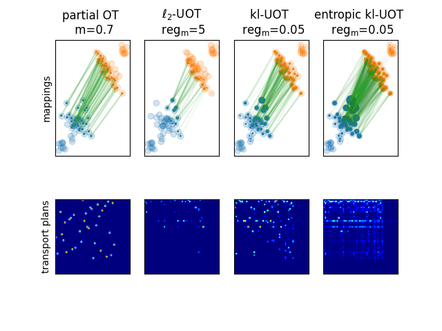
Plot the results

pl.figure(2)
transp = [partial_ot, l2_uot, kl_uot, entropic_kl_uot]
title = ["partial OT \n m=" + str(mass), "$\ell_2$-UOT \n $\mathrm{reg_m}$=" +
         str(reg_m_l2), "kl-UOT \n $\mathrm{reg_m}$=" + str(reg_m_kl),
         "entropic kl-UOT \n $\mathrm{reg_m}$=" + str(reg_m_kl)]

for p in range(4):
    pl.subplot(2, 4, p + 1)
    P = transp[p]
    if P.sum() > 0:
        P = P / P.max()
    for i in range(n):
        for j in range(n):
            if P[i, j] > 0:
                pl.plot([xs[i, 0], xt[j, 0]], [xs[i, 1], xt[j, 1]], color='C2',
                        alpha=P[i, j] * 0.3)
    pl.scatter(xs[:, 0], xs[:, 1], c='C0', alpha=0.2)
    pl.scatter(xt[:, 0], xt[:, 1], c='C1', alpha=0.2)
    pl.scatter(xs[:, 0], xs[:, 1], c='C0', s=P.sum(1).ravel() * (1 + p) * 2)
    pl.scatter(xt[:, 0], xt[:, 1], c='C1', s=P.sum(0).ravel() * (1 + p) * 2)
    pl.title(title[p])
    pl.yticks(())
    pl.xticks(())
    if p < 1:
        pl.ylabel("mappings")
    pl.subplot(2, 4, p + 5)
    pl.imshow(P, cmap='jet')
    pl.yticks(())
    pl.xticks(())
    if p < 1:
        pl.ylabel("transport plans")
pl.show()