Optimal transport with factored couplings

Illustration of the factored coupling OT between 2D empirical distributions

# Author: Remi Flamary <remi.flamary@polytechnique.edu>
#
# License: MIT License

# sphinx_gallery_thumbnail_number = 2

import numpy as np
import matplotlib.pylab as pl
import ot
import ot.plot

Generate data an plot it

# parameters and data generation

np.random.seed(42)

n = 100  # nb samples

xs = np.random.rand(n, 2) - .5

xs = xs + np.sign(xs)

xt = np.random.rand(n, 2) - .5

a, b = ot.unif(n), ot.unif(n)  # uniform distribution on samples

pl.figure(1)
pl.plot(xs[:, 0], xs[:, 1], '+b', label='Source samples')
pl.plot(xt[:, 0], xt[:, 1], 'xr', label='Target samples')
pl.legend(loc=0)
pl.title('Source and target distributions')

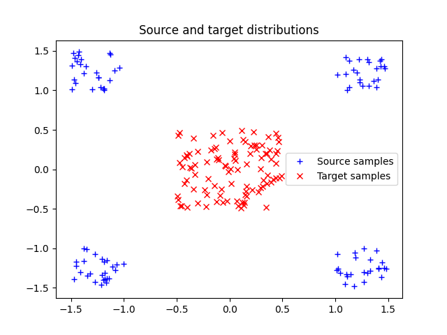
Text(0.5, 1.0, 'Source and target distributions')

Compute Factored OT and exact OT solutions

M = ot.dist(xs, xt)
G0 = ot.emd(a, b, M)

Ga, Gb, xb = ot.factored_optimal_transport(xs, xt, a, b, r=4)

Plot factored OT and exact OT solutions

pl.figure(2, (14, 4))

pl.subplot(1, 3, 1)
ot.plot.plot2D_samples_mat(xs, xt, G0, c=[.2, .2, .2], alpha=0.1)
pl.plot(xs[:, 0], xs[:, 1], '+b', label='Source samples')
pl.plot(xt[:, 0], xt[:, 1], 'xr', label='Target samples')
pl.title('Exact OT with samples')

pl.subplot(1, 3, 2)
ot.plot.plot2D_samples_mat(xs, xb, Ga, c=[.6, .6, .9], alpha=0.5)
ot.plot.plot2D_samples_mat(xb, xt, Gb, c=[.9, .6, .6], alpha=0.5)
pl.plot(xs[:, 0], xs[:, 1], '+b', label='Source samples')
pl.plot(xt[:, 0], xt[:, 1], 'xr', label='Target samples')
pl.plot(xb[:, 0], xb[:, 1], 'og', label='Template samples')
pl.title('Factored OT with template samples')

pl.subplot(1, 3, 3)
ot.plot.plot2D_samples_mat(xs, xt, Ga.dot(Gb), c=[.2, .2, .2], alpha=0.1)
pl.plot(xs[:, 0], xs[:, 1], '+b', label='Source samples')
pl.plot(xt[:, 0], xt[:, 1], 'xr', label='Target samples')
pl.title('Factored OT low rank OT plan')

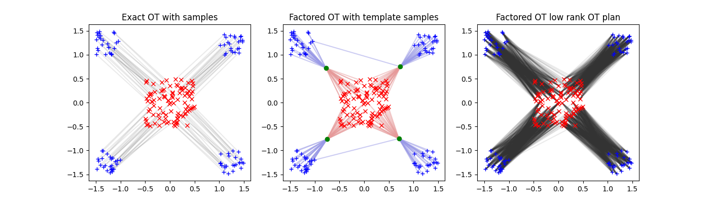
Text(0.5, 1.0, 'Factored OT low rank OT plan')