Note
Go to the end to download the full example code.
Stochastic examples
This example is designed to show how to use the stochastic optimization algorithms for discrete and semi-continuous measures from the POT library.
[18] Genevay, A., Cuturi, M., Peyré, G. & Bach, F. Stochastic Optimization for Large-scale Optimal Transport. Advances in Neural Information Processing Systems (2016).
[19] Seguy, V., Bhushan Damodaran, B., Flamary, R., Courty, N., Rolet, A. & Blondel, M. Large-scale Optimal Transport and Mapping Estimation. International Conference on Learning Representation (2018)
# Author: Kilian Fatras <kilian.fatras@gmail.com>
#
# License: MIT License

import matplotlib.pylab as pl
import numpy as np
import ot
import ot.plot
Compute the Transportation Matrix for the Semi-Dual Problem
Discrete case
Sample two discrete measures for the discrete case and compute their cost matrix c.
Call the “SAG” method to find the transportation matrix in the discrete case
method = "SAG"
sag_pi = ot.stochastic.solve_semi_dual_entropic(a, b, M, reg, method, numItermax)
print(sag_pi)
[[2.55553509e-02 9.96395660e-02 1.76579142e-02 4.31178196e-06]
 [1.21640234e-01 1.25357448e-02 1.30225078e-03 7.37891338e-03]
 [3.56123975e-03 7.61451746e-02 6.31505947e-02 1.33831456e-07]
 [2.61515202e-02 3.34246014e-02 8.28734709e-02 4.07550428e-04]
 [9.85500870e-03 7.52288517e-04 1.08262628e-02 1.21423583e-01]
 [2.16904253e-02 9.03825797e-04 1.87178503e-03 1.18391107e-01]
 [4.15462212e-02 2.65987989e-02 7.23177216e-02 2.39440107e-03]]
Semi-Continuous Case
Sample one general measure a, one discrete measures b for the semicontinuous case, the points where source and target measures are defined and compute the cost matrix.
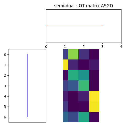
Call the “ASGD” method to find the transportation matrix in the semicontinuous case.
[3.89418541 7.69191648 3.88798203 2.63066822 1.4605918  3.30128899
 2.76039982] [-2.55838411 -2.42317354 -0.84802459  5.82958224]
[[2.36658434e-02 1.00210228e-01 1.89765631e-02 4.50856086e-06]
 [1.19762224e-01 1.34039510e-02 1.48790516e-03 8.20306258e-03]
 [3.18880498e-03 7.40472984e-02 6.56209042e-02 1.35308774e-07]
 [2.34839063e-02 3.25971567e-02 8.63628461e-02 4.13233727e-04]
 [8.78057873e-03 7.27931720e-04 1.11939332e-02 1.22154699e-01]
 [1.95469897e-02 8.84579013e-04 1.95751817e-03 1.20468056e-01]
 [3.77891909e-02 2.62747246e-02 7.63341399e-02 2.45908742e-03]]
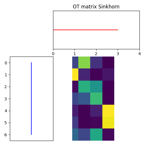
Compare the results with the Sinkhorn algorithm
sinkhorn_pi = ot.sinkhorn(a, b, M, reg)
print(sinkhorn_pi)
[[2.55553508e-02 9.96395661e-02 1.76579142e-02 4.31178193e-06]
 [1.21640234e-01 1.25357448e-02 1.30225079e-03 7.37891333e-03]
 [3.56123974e-03 7.61451746e-02 6.31505947e-02 1.33831455e-07]
 [2.61515201e-02 3.34246014e-02 8.28734709e-02 4.07550425e-04]
 [9.85500876e-03 7.52288523e-04 1.08262629e-02 1.21423583e-01]
 [2.16904255e-02 9.03825804e-04 1.87178504e-03 1.18391107e-01]
 [4.15462212e-02 2.65987989e-02 7.23177217e-02 2.39440105e-03]]
Plot Transportation Matrices
For SAG
pl.figure(4, figsize=(5, 5))
ot.plot.plot1D_mat(a, b, sag_pi, "semi-dual : OT matrix SAG")
pl.show()

For ASGD
pl.figure(4, figsize=(5, 5))
ot.plot.plot1D_mat(a, b, asgd_pi, "semi-dual : OT matrix ASGD")
pl.show()
For Sinkhorn
pl.figure(4, figsize=(5, 5))
ot.plot.plot1D_mat(a, b, sinkhorn_pi, "OT matrix Sinkhorn")
pl.show()

Compute the Transportation Matrix for the Dual Problem
Semi-continuous case
Sample one general measure a, one discrete measures b for the semi-continuous case and compute the cost matrix c.
n_source = 7
n_target = 4
reg = 1
numItermax = 100000
lr = 0.1
batch_size = 3
log = True

a = ot.utils.unif(n_source)
b = ot.utils.unif(n_target)

rng = np.random.RandomState(0)
X_source = rng.randn(n_source, 2)
Y_target = rng.randn(n_target, 2)
M = ot.dist(X_source, Y_target)
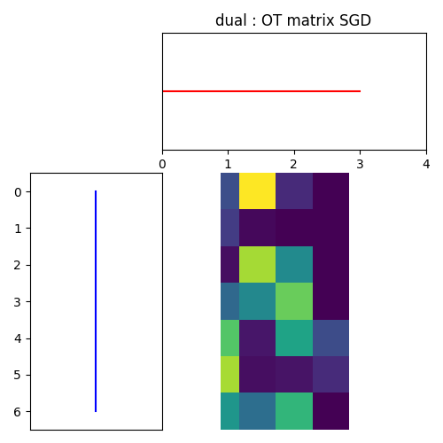
Call the “SGD” dual method to find the transportation matrix in the semi-continuous case
sgd_dual_pi, log_sgd = ot.stochastic.solve_dual_entropic(
    a, b, M, reg, batch_size, numItermax, lr, log=log
)
print(log_sgd["alpha"], log_sgd["beta"])
print(sgd_dual_pi)
[0.91165603 2.77176512 1.06822819 0.02120131 0.6126745  1.82423613
 0.11278947] [0.33918268 0.47789947 1.5719034  4.9335652 ]
[[2.17381811e-02 9.23710741e-02 1.08114235e-02 9.32409360e-08]
 [1.58461053e-02 1.77974690e-03 1.22107416e-04 2.44369039e-05]
 [3.44684454e-03 8.03203669e-02 4.39946687e-02 3.29296540e-09]
 [3.13249603e-02 4.36337600e-02 7.14514820e-02 1.24103327e-05]
 [6.81827650e-02 5.67237379e-03 5.39135941e-02 2.13564527e-02]
 [8.09098220e-02 3.67435169e-03 5.02563876e-03 1.12269228e-02]
 [4.85201684e-02 3.38544380e-02 6.07907676e-02 7.10879755e-05]]
Compare the results with the Sinkhorn algorithm
Call the Sinkhorn algorithm from POT
sinkhorn_pi = ot.sinkhorn(a, b, M, reg)
print(sinkhorn_pi)
[[2.55553508e-02 9.96395661e-02 1.76579142e-02 4.31178193e-06]
 [1.21640234e-01 1.25357448e-02 1.30225079e-03 7.37891333e-03]
 [3.56123974e-03 7.61451746e-02 6.31505947e-02 1.33831455e-07]
 [2.61515201e-02 3.34246014e-02 8.28734709e-02 4.07550425e-04]
 [9.85500876e-03 7.52288523e-04 1.08262629e-02 1.21423583e-01]
 [2.16904255e-02 9.03825804e-04 1.87178504e-03 1.18391107e-01]
 [4.15462212e-02 2.65987989e-02 7.23177217e-02 2.39440105e-03]]
Plot Transportation Matrices
For SGD
pl.figure(4, figsize=(5, 5))
ot.plot.plot1D_mat(a, b, sgd_dual_pi, "dual : OT matrix SGD")
pl.show()
For Sinkhorn
pl.figure(4, figsize=(5, 5))
ot.plot.plot1D_mat(a, b, sinkhorn_pi, "OT matrix Sinkhorn")
pl.show()
Total running time of the script: (0 minutes 6.580 seconds)