ot.stochastic

Stochastic solvers for regularized OT.

Functions

ot.stochastic.averaged_sgd_entropic_transport(a, b, M, reg, numItermax=300000, lr=None, random_state=None)

Compute the ASGD algorithm to solve the regularized semi continuous measures optimal transport max problem

The function solves the following optimization problem:

\[ \begin{align}\begin{aligned}\gamma = \mathop{\arg \min}_\gamma \quad \langle \gamma, \mathbf{M} \rangle_F + \mathrm{reg}\cdot\Omega(\gamma)\\s.t. \gamma \mathbf{1} = \mathbf{a}\\ \gamma^T \mathbf{1} = \mathbf{b}\\ \gamma \geq 0\end{aligned}\end{align} \]

Where :

• \(\mathbf{M}\) is the (ns, nt) metric cost matrix

• \(\Omega\) is the entropic regularization term with \(\Omega(\gamma)=\sum_{i,j} \gamma_{i,j}\log(\gamma_{i,j})\)

• \(\mathbf{a}\) and \(\mathbf{b}\) are source and target weights (sum to 1)

The algorithm used for solving the problem is the ASGD algorithm as proposed in [18] [alg.2]

Parameters:

• b (ndarray, shape (nt,)) – target measure

• M (ndarray, shape (ns, nt)) – cost matrix

• reg (float) – Regularization term > 0

• numItermax (int) – Number of iteration.

• lr (float) – Learning rate.

• random_state (int, RandomState instance or None, default=None) – Determines random number generation. Pass an int for reproducible output across multiple function calls.

Returns:

• ave_v (ndarray, shape (nt,)) – dual variable

• .. _references-averaged-sgd-entropic-transport

References

[18]

Genevay, A., Cuturi, M., Peyré, G. & Bach, F. (2016) Stochastic Optimization for Large-scale Optimal Transport. Advances in Neural Information Processing Systems (2016).

ot.stochastic.batch_grad_dual(a, b, M, reg, alpha, beta, batch_size, batch_alpha, batch_beta)

Computes the partial gradient of the dual optimal transport problem.

For each \((i,j)\) in a batch of coordinates, the partial gradients are :

\[ \begin{align}\begin{aligned}\partial_{\mathbf{u}_i} F = \frac{b_s}{l_v} \mathbf{u}_i - \sum_{j \in B_v} \mathbf{a}_i \mathbf{b}_j \exp\left( \frac{\mathbf{u}_i + \mathbf{v}_j - \mathbf{M}_{i,j}}{\mathrm{reg}} \right)\\\partial_{\mathbf{v}_j} F = \frac{b_s}{l_u} \mathbf{v}_j - \sum_{i \in B_u} \mathbf{a}_i \mathbf{b}_j \exp\left( \frac{\mathbf{u}_i + \mathbf{v}_j - \mathbf{M}_{i,j}}{\mathrm{reg}} \right)\end{aligned}\end{align} \]

Where :

• \(\mathbf{M}\) is the (ns, nt) metric cost matrix

• \(\mathbf{u}\), \(\mathbf{v}\) are dual variables in \(\mathbb{R}^{ns} \times \mathbb{R}^{nt}\)

• reg is the regularization term

• \(B_u\) and \(B_v\) are lists of index

• \(b_s\) is the size of the batches \(B_u\) and \(B_v\)

• \(l_u\) and \(l_v\) are the lengths of \(B_u\) and \(B_v\)

• \(\mathbf{a}\) and \(\mathbf{b}\) are source and target weights (sum to 1)

The algorithm used for solving the dual problem is the SGD algorithm as proposed in [19] [alg.1]

Parameters:

• a (ndarray, shape (ns,)) – source measure

• b (ndarray, shape (nt,)) – target measure

• M (ndarray, shape (ns, nt)) – cost matrix

• reg (float) – Regularization term > 0

• alpha (ndarray, shape (ns,)) – dual variable

• beta (ndarray, shape (nt,)) – dual variable

• batch_size (int) – size of the batch

• batch_alpha (ndarray, shape (bs,)) – batch of index of alpha

• batch_beta (ndarray, shape (bs,)) – batch of index of beta

Returns:

• grad (ndarray, shape (ns,)) – partial grad F

• .. _references-batch-grad-dual

References

[19]

Seguy, V., Bhushan Damodaran, B., Flamary, R., Courty, N., Rolet, A.& Blondel, M. Large-scale Optimal Transport and Mapping Estimation. International Conference on Learning Representation (2018)

ot.stochastic.c_transform_entropic(b, M, reg, beta)

The goal is to recover u from the c-transform.

The function computes the c-transform of a dual variable from the other dual variable:

\[\mathbf{u} = \mathbf{v}^{c,reg} = - \mathrm{reg} \sum_j \mathbf{b}_j \exp\left( \frac{\mathbf{v} - \mathbf{M}}{\mathrm{reg}} \right)\]

Where :

• \(\mathbf{M}\) is the (ns, nt) metric cost matrix

• \(\mathbf{u}\), \(\mathbf{v}\) are dual variables in \(\mathbb{R}^{ns} \times \mathbb{R}^{nt}\)

• reg is the regularization term

It is used to recover an optimal u from optimal v solving the semi dual problem, see Proposition 2.1 of [18]

Parameters:

• b (ndarray, shape (nt,)) – Target measure

• M (ndarray, shape (ns, nt)) – Cost matrix

• reg (float) – Regularization term > 0

• v (ndarray, shape (nt,)) – Dual variable.

Returns:

• u (ndarray, shape (ns,)) – Dual variable.

• .. _references-c-transform-entropic

References

[18]

Genevay, A., Cuturi, M., Peyré, G. & Bach, F. (2016) Stochastic Optimization for Large-scale Optimal Transport. Advances in Neural Information Processing Systems (2016).

ot.stochastic.coordinate_grad_semi_dual(b, M, reg, beta, i)

Compute the coordinate gradient update for regularized discrete distributions for \((i, :)\)

The function computes the gradient of the semi dual problem:

\[\max_\mathbf{v} \ \sum_i \mathbf{a}_i \left[ \sum_j \mathbf{v}_j \mathbf{b}_j - \mathrm{reg} \cdot \log \left( \sum_j \mathbf{b}_j \exp \left( \frac{\mathbf{v}_j - \mathbf{M}_{i,j}}{\mathrm{reg}} \right) \right) \right]\]

Where :

• \(\mathbf{M}\) is the (ns, nt) metric cost matrix

• \(\mathbf{v}\) is a dual variable in \(\mathbb{R}^{nt}\)

• reg is the regularization term

• \(\mathbf{a}\) and \(\mathbf{b}\) are source and target weights (sum to 1)

The algorithm used for solving the problem is the ASGD & SAG algorithms as proposed in [18] [alg.1 & alg.2]

Parameters:

• b (ndarray, shape (nt,)) – Target measure.

• M (ndarray, shape (ns, nt)) – Cost matrix.

• reg (float) – Regularization term > 0.

• v (ndarray, shape (nt,)) – Dual variable.

• i (int) – Picked number i.

Returns:

• coordinate gradient (ndarray, shape (nt,))

• .. _references-coordinate-grad-semi-dual

References

[18]

Genevay, A., Cuturi, M., Peyré, G. & Bach, F. (2016) Stochastic Optimization for Large-scale Optimal Transport. Advances in Neural Information Processing Systems (2016).

ot.stochastic.loss_dual_entropic(u, v, xs, xt, reg=1, ws=None, wt=None, metric='sqeuclidean')

Compute the dual loss of the entropic OT as in equation (6)-(7) of [19]

This loss is backend compatible and can be used for stochastic optimization of the dual potentials. It can be used on the full dataset (beware of memory) or on minibatches.

Parameters:

• u (array-like, shape (ns,)) – Source dual potential

• v (array-like, shape (nt,)) – Target dual potential

• xs (array-like, shape (ns,d)) – Source samples

• xt (array-like, shape (ns,d)) – Target samples

• reg (float) – Regularization term > 0 (default=1)

• ws (array-like, shape (ns,), optional) – Source sample weights (default unif)

• wt (array-like, shape (ns,), optional) – Target sample weights (default unif)

• metric (string, callable) – Ground metric for OT (default quadratic). Can be given as a callable function taking (xs,xt) as parameters.

Returns:

dual_loss – Dual loss (to maximize)

Return type:

array-like

References

[19]

Seguy, V., Bhushan Damodaran, B., Flamary, R., Courty, N., Rolet, A.& Blondel, M. Large-scale Optimal Transport and Mapping Estimation. International Conference on Learning Representation (2018)

Examples using ot.stochastic.loss_dual_entropic

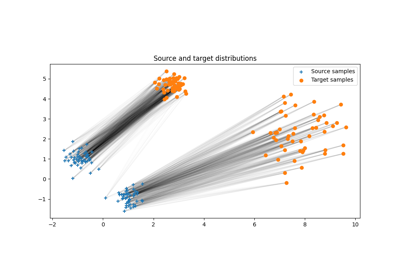
Dual OT solvers for entropic and quadratic regularized OT with Pytorch

Dual OT solvers for entropic and quadratic regularized OT with Pytorch

Continuous OT plan estimation with Pytorch

Continuous OT plan estimation with Pytorch

ot.stochastic.loss_dual_quadratic(u, v, xs, xt, reg=1, ws=None, wt=None, metric='sqeuclidean')

Compute the dual loss of the quadratic regularized OT as in equation (6)-(7) of [19]

This loss is backend compatible and can be used for stochastic optimization of the dual potentials. It can be used on the full dataset (beware of memory) or on minibatches.

Parameters:

• u (array-like, shape (ns,)) – Source dual potential

• v (array-like, shape (nt,)) – Target dual potential

• xs (array-like, shape (ns,d)) – Source samples

• xt (array-like, shape (ns,d)) – Target samples

• reg (float) – Regularization term > 0 (default=1)

• ws (array-like, shape (ns,), optional) – Source sample weights (default unif)

• wt (array-like, shape (ns,), optional) – Target sample weights (default unif)

• metric (string, callable) – Ground metric for OT (default quadratic). Can be given as a callable function taking (xs,xt) as parameters.

Returns:

dual_loss – Dual loss (to maximize)

Return type:

array-like

References

[19]

Seguy, V., Bhushan Damodaran, B., Flamary, R., Courty, N., Rolet, A.& Blondel, M. Large-scale Optimal Transport and Mapping Estimation. International Conference on Learning Representation (2018)

Examples using ot.stochastic.loss_dual_quadratic

Dual OT solvers for entropic and quadratic regularized OT with Pytorch

Dual OT solvers for entropic and quadratic regularized OT with Pytorch

ot.stochastic.plan_dual_entropic(u, v, xs, xt, reg=1, ws=None, wt=None, metric='sqeuclidean')

Compute the primal OT plan the entropic OT as in equation (8) of [19]

This loss is backend compatible and can be used for stochastic optimization of the dual potentials. It can be used on the full dataset (beware of memory) or on minibatches.

Parameters:

• u (array-like, shape (ns,)) – Source dual potential

• v (array-like, shape (nt,)) – Target dual potential

• xs (array-like, shape (ns,d)) – Source samples

• xt (array-like, shape (ns,d)) – Target samples

• reg (float) – Regularization term > 0 (default=1)

• ws (array-like, shape (ns,), optional) – Source sample weights (default unif)

• wt (array-like, shape (ns,), optional) – Target sample weights (default unif)

• metric (string, callable) – Ground metric for OT (default quadratic). Can be given as a callable function taking (xs,xt) as parameters.

Returns:

G – Primal OT plan

Return type:

array-like

References

[19]

Seguy, V., Bhushan Damodaran, B., Flamary, R., Courty, N., Rolet, A.& Blondel, M. Large-scale Optimal Transport and Mapping Estimation. International Conference on Learning Representation (2018)

Examples using ot.stochastic.plan_dual_entropic

Dual OT solvers for entropic and quadratic regularized OT with Pytorch

Dual OT solvers for entropic and quadratic regularized OT with Pytorch

Continuous OT plan estimation with Pytorch

Continuous OT plan estimation with Pytorch

ot.stochastic.plan_dual_quadratic(u, v, xs, xt, reg=1, ws=None, wt=None, metric='sqeuclidean')

Compute the primal OT plan the quadratic regularized OT as in equation (8) of [19]

This loss is backend compatible and can be used for stochastic optimization of the dual potentials. It can be used on the full dataset (beware of memory) or on minibatches.

Parameters:

• u (array-like, shape (ns,)) – Source dual potential

• v (array-like, shape (nt,)) – Target dual potential

• xs (array-like, shape (ns,d)) – Source samples

• xt (array-like, shape (ns,d)) – Target samples

• reg (float) – Regularization term > 0 (default=1)

• ws (array-like, shape (ns,), optional) – Source sample weights (default unif)

• wt (array-like, shape (ns,), optional) – Target sample weights (default unif)

• metric (string, callable) – Ground metric for OT (default quadratic). Can be given as a callable function taking (xs,xt) as parameters.

Returns:

G – Primal OT plan

Return type:

array-like

References

[19]

Seguy, V., Bhushan Damodaran, B., Flamary, R., Courty, N., Rolet, A.& Blondel, M. Large-scale Optimal Transport and Mapping Estimation. International Conference on Learning Representation (2018)

Examples using ot.stochastic.plan_dual_quadratic

Dual OT solvers for entropic and quadratic regularized OT with Pytorch

Dual OT solvers for entropic and quadratic regularized OT with Pytorch

ot.stochastic.sag_entropic_transport(a, b, M, reg, numItermax=10000, lr=None, random_state=None)

Compute the SAG algorithm to solve the regularized discrete measures optimal transport max problem

The function solves the following optimization problem:

\[ \begin{align}\begin{aligned}\gamma = \mathop{\arg \min}_\gamma \quad \langle \gamma, \mathbf{M} \rangle_F + \mathrm{reg} \cdot\Omega(\gamma)\\s.t. \ \gamma \mathbf{1} = \mathbf{a}\\ \gamma^T \mathbf{1} = \mathbf{b}\\ \gamma \geq 0\end{aligned}\end{align} \]

Where :

• \(\mathbf{M}\) is the (ns, nt) metric cost matrix

• \(\Omega\) is the entropic regularization term with \(\Omega(\gamma)=\sum_{i,j} \gamma_{i,j}\log(\gamma_{i,j})\)

• \(\mathbf{a}\) and \(\mathbf{b}\) are source and target weights (sum to 1)

The algorithm used for solving the problem is the SAG algorithm as proposed in [18] [alg.1]

Parameters:

• a (ndarray, shape (ns,),) – Source measure.

• b (ndarray, shape (nt,),) – Target measure.

• M (ndarray, shape (ns, nt),) – Cost matrix.

• reg (float) – Regularization term > 0

• numItermax (int) – Number of iteration.

• lr (float) – Learning rate.

• random_state (int, RandomState instance or None, default=None) – Determines random number generation. Pass an int for reproducible output across multiple function calls.

Returns:

• v (ndarray, shape (nt,)) – Dual variable.

• .. _references-sag-entropic-transport

References

[18]

Genevay, A., Cuturi, M., Peyré, G. & Bach, F. (2016) Stochastic Optimization for Large-scale Optimal Transport. Advances in Neural Information Processing Systems (2016).

ot.stochastic.sgd_entropic_regularization(a, b, M, reg, batch_size, numItermax, lr, random_state=None)

Compute the sgd algorithm to solve the regularized discrete measures optimal transport dual problem

The function solves the following optimization problem:

\[ \begin{align}\begin{aligned}\gamma = \mathop{\arg \min}_\gamma \quad \langle \gamma, \mathbf{M} \rangle_F + \mathrm{reg} \cdot\Omega(\gamma)\\s.t. \ \gamma \mathbf{1} = \mathbf{a}\\ \gamma^T \mathbf{1} = \mathbf{b}\\ \gamma \geq 0\end{aligned}\end{align} \]

Where :

• \(\mathbf{M}\) is the (ns, nt) metric cost matrix

• \(\Omega\) is the entropic regularization term with \(\Omega(\gamma)=\sum_{i,j} \gamma_{i,j}\log(\gamma_{i,j})\)

• \(\mathbf{a}\) and \(\mathbf{b}\) are source and target weights (sum to 1)

Parameters:

• a (ndarray, shape (ns,)) – source measure

• b (ndarray, shape (nt,)) – target measure

• M (ndarray, shape (ns, nt)) – cost matrix

• reg (float) – Regularization term > 0

• batch_size (int) – size of the batch

• numItermax (int) – number of iteration

• lr (float) – learning rate

• random_state (int, RandomState instance or None, default=None) – Determines random number generation. Pass an int for reproducible output across multiple function calls.

Returns:

• alpha (ndarray, shape (ns,)) – dual variable

• beta (ndarray, shape (nt,)) – dual variable

References

[19]

Seguy, V., Bhushan Damodaran, B., Flamary, R., Courty, N., Rolet, A.& Blondel, M. Large-scale Optimal Transport and Mapping Estimation. International Conference on Learning Representation (2018)

ot.stochastic.solve_dual_entropic(a, b, M, reg, batch_size, numItermax=10000, lr=1, log=False)

Compute the transportation matrix to solve the regularized discrete measures optimal transport dual problem

The function solves the following optimization problem:

\[ \begin{align}\begin{aligned}\gamma = \mathop{\arg \min}_\gamma \quad \langle \gamma, \mathbf{M} \rangle_F + \mathrm{reg} \cdot\Omega(\gamma)\\s.t. \ \gamma \mathbf{1} = \mathbf{a}\\ \gamma^T \mathbf{1} = \mathbf{b}\\ \gamma \geq 0\end{aligned}\end{align} \]

Where :

• \(\mathbf{M}\) is the (ns, nt) metric cost matrix

• \(\Omega\) is the entropic regularization term with \(\Omega(\gamma)=\sum_{i,j} \gamma_{i,j}\log(\gamma_{i,j})\)

• \(\mathbf{a}\) and \(\mathbf{b}\) are source and target weights (sum to 1)

Parameters:

• a (ndarray, shape (ns,)) – source measure

• b (ndarray, shape (nt,)) – target measure

• M (ndarray, shape (ns, nt)) – cost matrix

• reg (float) – Regularization term > 0

• batch_size (int) – size of the batch

• numItermax (int) – number of iteration

• lr (float) – learning rate

• log (bool, optional) – record log if True

Returns:

• pi (ndarray, shape (ns, nt)) – transportation matrix

• log (dict) – log dictionary return only if log==True in parameters

References

[19]

Seguy, V., Bhushan Damodaran, B., Flamary, R., Courty, N., Rolet, A.& Blondel, M. Large-scale Optimal Transport and Mapping Estimation. International Conference on Learning Representation (2018)

Examples using ot.stochastic.solve_dual_entropic

Stochastic examples

Stochastic examples

ot.stochastic.solve_semi_dual_entropic(a, b, M, reg, method, numItermax=10000, lr=None, log=False)

Compute the transportation matrix to solve the regularized discrete measures optimal transport max problem

The function solves the following optimization problem:

\[ \begin{align}\begin{aligned}\gamma = \mathop{\arg \min}_\gamma \quad \langle \gamma, \mathbf{M} \rangle_F + \mathrm{reg} \cdot\Omega(\gamma)\\s.t. \ \gamma \mathbf{1} = \mathbf{a}\\ \gamma^T \mathbf{1} = \mathbf{b}\\ \gamma \geq 0\end{aligned}\end{align} \]

Where :

• \(\mathbf{M}\) is the (ns, nt) metric cost matrix

• \(\Omega\) is the entropic regularization term with \(\Omega(\gamma)=\sum_{i,j} \gamma_{i,j}\log(\gamma_{i,j})\)

• \(\mathbf{a}\) and \(\mathbf{b}\) are source and target weights (sum to 1)

The algorithm used for solving the problem is the SAG or ASGD algorithms as proposed in [18]

Parameters:

• a (ndarray, shape (ns,)) – source measure

• b (ndarray, shape (nt,)) – target measure

• M (ndarray, shape (ns, nt)) – cost matrix

• reg (float) – Regularization term > 0

• method (str) – used method (SAG or ASGD)

• numItermax (int) – number of iteration

• lr (float) – learning rate

• n_source (int) – size of the source measure

• n_target (int) – size of the target measure

• log (bool, optional) – record log if True

Returns:

• pi (ndarray, shape (ns, nt)) – transportation matrix

• log (dict) – log dictionary return only if log==True in parameters

• .. _references-solve-semi-dual-entropic

References

[18]

Genevay, A., Cuturi, M., Peyré, G. & Bach, F. (2016) Stochastic Optimization for Large-scale Optimal Transport. Advances in Neural Information Processing Systems (2016).

Examples using ot.stochastic.solve_semi_dual_entropic

Stochastic examples

Stochastic examples

ot.stochastic.averaged_sgd_entropic_transport(a, b, M, reg, numItermax=300000, lr=None, random_state=None)

Compute the ASGD algorithm to solve the regularized semi continuous measures optimal transport max problem

The function solves the following optimization problem:

\[ \begin{align}\begin{aligned}\gamma = \mathop{\arg \min}_\gamma \quad \langle \gamma, \mathbf{M} \rangle_F + \mathrm{reg}\cdot\Omega(\gamma)\\s.t. \gamma \mathbf{1} = \mathbf{a}\\ \gamma^T \mathbf{1} = \mathbf{b}\\ \gamma \geq 0\end{aligned}\end{align} \]

Where :

• \(\mathbf{M}\) is the (ns, nt) metric cost matrix

• \(\Omega\) is the entropic regularization term with \(\Omega(\gamma)=\sum_{i,j} \gamma_{i,j}\log(\gamma_{i,j})\)

• \(\mathbf{a}\) and \(\mathbf{b}\) are source and target weights (sum to 1)

The algorithm used for solving the problem is the ASGD algorithm as proposed in [18] [alg.2]

Parameters:

• b (ndarray, shape (nt,)) – target measure

• M (ndarray, shape (ns, nt)) – cost matrix

• reg (float) – Regularization term > 0

• numItermax (int) – Number of iteration.

• lr (float) – Learning rate.

• random_state (int, RandomState instance or None, default=None) – Determines random number generation. Pass an int for reproducible output across multiple function calls.

Returns:

• ave_v (ndarray, shape (nt,)) – dual variable

• .. _references-averaged-sgd-entropic-transport

References

[18]

Genevay, A., Cuturi, M., Peyré, G. & Bach, F. (2016) Stochastic Optimization for Large-scale Optimal Transport. Advances in Neural Information Processing Systems (2016).

ot.stochastic.batch_grad_dual(a, b, M, reg, alpha, beta, batch_size, batch_alpha, batch_beta)

Computes the partial gradient of the dual optimal transport problem.

For each \((i,j)\) in a batch of coordinates, the partial gradients are :

\[ \begin{align}\begin{aligned}\partial_{\mathbf{u}_i} F = \frac{b_s}{l_v} \mathbf{u}_i - \sum_{j \in B_v} \mathbf{a}_i \mathbf{b}_j \exp\left( \frac{\mathbf{u}_i + \mathbf{v}_j - \mathbf{M}_{i,j}}{\mathrm{reg}} \right)\\\partial_{\mathbf{v}_j} F = \frac{b_s}{l_u} \mathbf{v}_j - \sum_{i \in B_u} \mathbf{a}_i \mathbf{b}_j \exp\left( \frac{\mathbf{u}_i + \mathbf{v}_j - \mathbf{M}_{i,j}}{\mathrm{reg}} \right)\end{aligned}\end{align} \]

Where :

• \(\mathbf{M}\) is the (ns, nt) metric cost matrix

• \(\mathbf{u}\), \(\mathbf{v}\) are dual variables in \(\mathbb{R}^{ns} \times \mathbb{R}^{nt}\)

• reg is the regularization term

• \(B_u\) and \(B_v\) are lists of index

• \(b_s\) is the size of the batches \(B_u\) and \(B_v\)

• \(l_u\) and \(l_v\) are the lengths of \(B_u\) and \(B_v\)

• \(\mathbf{a}\) and \(\mathbf{b}\) are source and target weights (sum to 1)

The algorithm used for solving the dual problem is the SGD algorithm as proposed in [19] [alg.1]

Parameters:

• a (ndarray, shape (ns,)) – source measure

• b (ndarray, shape (nt,)) – target measure

• M (ndarray, shape (ns, nt)) – cost matrix

• reg (float) – Regularization term > 0

• alpha (ndarray, shape (ns,)) – dual variable

• beta (ndarray, shape (nt,)) – dual variable

• batch_size (int) – size of the batch

• batch_alpha (ndarray, shape (bs,)) – batch of index of alpha

• batch_beta (ndarray, shape (bs,)) – batch of index of beta

Returns:

• grad (ndarray, shape (ns,)) – partial grad F

• .. _references-batch-grad-dual

References

[19]

Seguy, V., Bhushan Damodaran, B., Flamary, R., Courty, N., Rolet, A.& Blondel, M. Large-scale Optimal Transport and Mapping Estimation. International Conference on Learning Representation (2018)

ot.stochastic.c_transform_entropic(b, M, reg, beta)

The goal is to recover u from the c-transform.

The function computes the c-transform of a dual variable from the other dual variable:

\[\mathbf{u} = \mathbf{v}^{c,reg} = - \mathrm{reg} \sum_j \mathbf{b}_j \exp\left( \frac{\mathbf{v} - \mathbf{M}}{\mathrm{reg}} \right)\]

Where :

• \(\mathbf{M}\) is the (ns, nt) metric cost matrix

• \(\mathbf{u}\), \(\mathbf{v}\) are dual variables in \(\mathbb{R}^{ns} \times \mathbb{R}^{nt}\)

• reg is the regularization term

It is used to recover an optimal u from optimal v solving the semi dual problem, see Proposition 2.1 of [18]

Parameters:

• b (ndarray, shape (nt,)) – Target measure

• M (ndarray, shape (ns, nt)) – Cost matrix

• reg (float) – Regularization term > 0

• v (ndarray, shape (nt,)) – Dual variable.

Returns:

• u (ndarray, shape (ns,)) – Dual variable.

• .. _references-c-transform-entropic

References

[18]

Genevay, A., Cuturi, M., Peyré, G. & Bach, F. (2016) Stochastic Optimization for Large-scale Optimal Transport. Advances in Neural Information Processing Systems (2016).

ot.stochastic.coordinate_grad_semi_dual(b, M, reg, beta, i)

Compute the coordinate gradient update for regularized discrete distributions for \((i, :)\)

The function computes the gradient of the semi dual problem:

\[\max_\mathbf{v} \ \sum_i \mathbf{a}_i \left[ \sum_j \mathbf{v}_j \mathbf{b}_j - \mathrm{reg} \cdot \log \left( \sum_j \mathbf{b}_j \exp \left( \frac{\mathbf{v}_j - \mathbf{M}_{i,j}}{\mathrm{reg}} \right) \right) \right]\]

Where :

• \(\mathbf{M}\) is the (ns, nt) metric cost matrix

• \(\mathbf{v}\) is a dual variable in \(\mathbb{R}^{nt}\)

• reg is the regularization term

• \(\mathbf{a}\) and \(\mathbf{b}\) are source and target weights (sum to 1)

The algorithm used for solving the problem is the ASGD & SAG algorithms as proposed in [18] [alg.1 & alg.2]

Parameters:

• b (ndarray, shape (nt,)) – Target measure.

• M (ndarray, shape (ns, nt)) – Cost matrix.

• reg (float) – Regularization term > 0.

• v (ndarray, shape (nt,)) – Dual variable.

• i (int) – Picked number i.

Returns:

• coordinate gradient (ndarray, shape (nt,))

• .. _references-coordinate-grad-semi-dual

References

[18]

Genevay, A., Cuturi, M., Peyré, G. & Bach, F. (2016) Stochastic Optimization for Large-scale Optimal Transport. Advances in Neural Information Processing Systems (2016).

ot.stochastic.loss_dual_entropic(u, v, xs, xt, reg=1, ws=None, wt=None, metric='sqeuclidean')

Compute the dual loss of the entropic OT as in equation (6)-(7) of [19]

This loss is backend compatible and can be used for stochastic optimization of the dual potentials. It can be used on the full dataset (beware of memory) or on minibatches.

Parameters:

• u (array-like, shape (ns,)) – Source dual potential

• v (array-like, shape (nt,)) – Target dual potential

• xs (array-like, shape (ns,d)) – Source samples

• xt (array-like, shape (ns,d)) – Target samples

• reg (float) – Regularization term > 0 (default=1)

• ws (array-like, shape (ns,), optional) – Source sample weights (default unif)

• wt (array-like, shape (ns,), optional) – Target sample weights (default unif)

• metric (string, callable) – Ground metric for OT (default quadratic). Can be given as a callable function taking (xs,xt) as parameters.

Returns:

dual_loss – Dual loss (to maximize)

Return type:

array-like

References

[19]

Seguy, V., Bhushan Damodaran, B., Flamary, R., Courty, N., Rolet, A.& Blondel, M. Large-scale Optimal Transport and Mapping Estimation. International Conference on Learning Representation (2018)

ot.stochastic.loss_dual_quadratic(u, v, xs, xt, reg=1, ws=None, wt=None, metric='sqeuclidean')

Compute the dual loss of the quadratic regularized OT as in equation (6)-(7) of [19]

This loss is backend compatible and can be used for stochastic optimization of the dual potentials. It can be used on the full dataset (beware of memory) or on minibatches.

Parameters:

• u (array-like, shape (ns,)) – Source dual potential

• v (array-like, shape (nt,)) – Target dual potential

• xs (array-like, shape (ns,d)) – Source samples

• xt (array-like, shape (ns,d)) – Target samples

• reg (float) – Regularization term > 0 (default=1)

• ws (array-like, shape (ns,), optional) – Source sample weights (default unif)

• wt (array-like, shape (ns,), optional) – Target sample weights (default unif)

• metric (string, callable) – Ground metric for OT (default quadratic). Can be given as a callable function taking (xs,xt) as parameters.

Returns:

dual_loss – Dual loss (to maximize)

Return type:

array-like

References

[19]

Seguy, V., Bhushan Damodaran, B., Flamary, R., Courty, N., Rolet, A.& Blondel, M. Large-scale Optimal Transport and Mapping Estimation. International Conference on Learning Representation (2018)

ot.stochastic.plan_dual_entropic(u, v, xs, xt, reg=1, ws=None, wt=None, metric='sqeuclidean')

Compute the primal OT plan the entropic OT as in equation (8) of [19]

This loss is backend compatible and can be used for stochastic optimization of the dual potentials. It can be used on the full dataset (beware of memory) or on minibatches.

Parameters:

• u (array-like, shape (ns,)) – Source dual potential

• v (array-like, shape (nt,)) – Target dual potential

• xs (array-like, shape (ns,d)) – Source samples

• xt (array-like, shape (ns,d)) – Target samples

• reg (float) – Regularization term > 0 (default=1)

• ws (array-like, shape (ns,), optional) – Source sample weights (default unif)

• wt (array-like, shape (ns,), optional) – Target sample weights (default unif)

• metric (string, callable) – Ground metric for OT (default quadratic). Can be given as a callable function taking (xs,xt) as parameters.

Returns:

G – Primal OT plan

Return type:

array-like

References

[19]

Seguy, V., Bhushan Damodaran, B., Flamary, R., Courty, N., Rolet, A.& Blondel, M. Large-scale Optimal Transport and Mapping Estimation. International Conference on Learning Representation (2018)

ot.stochastic.plan_dual_quadratic(u, v, xs, xt, reg=1, ws=None, wt=None, metric='sqeuclidean')

Compute the primal OT plan the quadratic regularized OT as in equation (8) of [19]

This loss is backend compatible and can be used for stochastic optimization of the dual potentials. It can be used on the full dataset (beware of memory) or on minibatches.

Parameters:

• u (array-like, shape (ns,)) – Source dual potential

• v (array-like, shape (nt,)) – Target dual potential

• xs (array-like, shape (ns,d)) – Source samples

• xt (array-like, shape (ns,d)) – Target samples

• reg (float) – Regularization term > 0 (default=1)

• ws (array-like, shape (ns,), optional) – Source sample weights (default unif)

• wt (array-like, shape (ns,), optional) – Target sample weights (default unif)

• metric (string, callable) – Ground metric for OT (default quadratic). Can be given as a callable function taking (xs,xt) as parameters.

Returns:

G – Primal OT plan

Return type:

array-like

References

[19]

Seguy, V., Bhushan Damodaran, B., Flamary, R., Courty, N., Rolet, A.& Blondel, M. Large-scale Optimal Transport and Mapping Estimation. International Conference on Learning Representation (2018)

ot.stochastic.sag_entropic_transport(a, b, M, reg, numItermax=10000, lr=None, random_state=None)

Compute the SAG algorithm to solve the regularized discrete measures optimal transport max problem

The function solves the following optimization problem:

\[ \begin{align}\begin{aligned}\gamma = \mathop{\arg \min}_\gamma \quad \langle \gamma, \mathbf{M} \rangle_F + \mathrm{reg} \cdot\Omega(\gamma)\\s.t. \ \gamma \mathbf{1} = \mathbf{a}\\ \gamma^T \mathbf{1} = \mathbf{b}\\ \gamma \geq 0\end{aligned}\end{align} \]

Where :

• \(\mathbf{M}\) is the (ns, nt) metric cost matrix

• \(\Omega\) is the entropic regularization term with \(\Omega(\gamma)=\sum_{i,j} \gamma_{i,j}\log(\gamma_{i,j})\)

• \(\mathbf{a}\) and \(\mathbf{b}\) are source and target weights (sum to 1)

The algorithm used for solving the problem is the SAG algorithm as proposed in [18] [alg.1]

Parameters:

• a (ndarray, shape (ns,),) – Source measure.

• b (ndarray, shape (nt,),) – Target measure.

• M (ndarray, shape (ns, nt),) – Cost matrix.

• reg (float) – Regularization term > 0

• numItermax (int) – Number of iteration.

• lr (float) – Learning rate.

• random_state (int, RandomState instance or None, default=None) – Determines random number generation. Pass an int for reproducible output across multiple function calls.

Returns:

• v (ndarray, shape (nt,)) – Dual variable.

• .. _references-sag-entropic-transport

References

[18]

Genevay, A., Cuturi, M., Peyré, G. & Bach, F. (2016) Stochastic Optimization for Large-scale Optimal Transport. Advances in Neural Information Processing Systems (2016).

ot.stochastic.sgd_entropic_regularization(a, b, M, reg, batch_size, numItermax, lr, random_state=None)

Compute the sgd algorithm to solve the regularized discrete measures optimal transport dual problem

The function solves the following optimization problem:

\[ \begin{align}\begin{aligned}\gamma = \mathop{\arg \min}_\gamma \quad \langle \gamma, \mathbf{M} \rangle_F + \mathrm{reg} \cdot\Omega(\gamma)\\s.t. \ \gamma \mathbf{1} = \mathbf{a}\\ \gamma^T \mathbf{1} = \mathbf{b}\\ \gamma \geq 0\end{aligned}\end{align} \]

Where :

• \(\mathbf{M}\) is the (ns, nt) metric cost matrix

• \(\Omega\) is the entropic regularization term with \(\Omega(\gamma)=\sum_{i,j} \gamma_{i,j}\log(\gamma_{i,j})\)

• \(\mathbf{a}\) and \(\mathbf{b}\) are source and target weights (sum to 1)

Parameters:

• a (ndarray, shape (ns,)) – source measure

• b (ndarray, shape (nt,)) – target measure

• M (ndarray, shape (ns, nt)) – cost matrix

• reg (float) – Regularization term > 0

• batch_size (int) – size of the batch

• numItermax (int) – number of iteration

• lr (float) – learning rate

• random_state (int, RandomState instance or None, default=None) – Determines random number generation. Pass an int for reproducible output across multiple function calls.

Returns:

• alpha (ndarray, shape (ns,)) – dual variable

• beta (ndarray, shape (nt,)) – dual variable

References

[19]

Seguy, V., Bhushan Damodaran, B., Flamary, R., Courty, N., Rolet, A.& Blondel, M. Large-scale Optimal Transport and Mapping Estimation. International Conference on Learning Representation (2018)

ot.stochastic.solve_dual_entropic(a, b, M, reg, batch_size, numItermax=10000, lr=1, log=False)

Compute the transportation matrix to solve the regularized discrete measures optimal transport dual problem

The function solves the following optimization problem:

\[ \begin{align}\begin{aligned}\gamma = \mathop{\arg \min}_\gamma \quad \langle \gamma, \mathbf{M} \rangle_F + \mathrm{reg} \cdot\Omega(\gamma)\\s.t. \ \gamma \mathbf{1} = \mathbf{a}\\ \gamma^T \mathbf{1} = \mathbf{b}\\ \gamma \geq 0\end{aligned}\end{align} \]

Where :

• \(\mathbf{M}\) is the (ns, nt) metric cost matrix

• \(\Omega\) is the entropic regularization term with \(\Omega(\gamma)=\sum_{i,j} \gamma_{i,j}\log(\gamma_{i,j})\)

• \(\mathbf{a}\) and \(\mathbf{b}\) are source and target weights (sum to 1)

Parameters:

• a (ndarray, shape (ns,)) – source measure

• b (ndarray, shape (nt,)) – target measure

• M (ndarray, shape (ns, nt)) – cost matrix

• reg (float) – Regularization term > 0

• batch_size (int) – size of the batch

• numItermax (int) – number of iteration

• lr (float) – learning rate

• log (bool, optional) – record log if True

Returns:

• pi (ndarray, shape (ns, nt)) – transportation matrix

• log (dict) – log dictionary return only if log==True in parameters

References

[19]

Seguy, V., Bhushan Damodaran, B., Flamary, R., Courty, N., Rolet, A.& Blondel, M. Large-scale Optimal Transport and Mapping Estimation. International Conference on Learning Representation (2018)

ot.stochastic.solve_semi_dual_entropic(a, b, M, reg, method, numItermax=10000, lr=None, log=False)

Compute the transportation matrix to solve the regularized discrete measures optimal transport max problem

The function solves the following optimization problem:

\[ \begin{align}\begin{aligned}\gamma = \mathop{\arg \min}_\gamma \quad \langle \gamma, \mathbf{M} \rangle_F + \mathrm{reg} \cdot\Omega(\gamma)\\s.t. \ \gamma \mathbf{1} = \mathbf{a}\\ \gamma^T \mathbf{1} = \mathbf{b}\\ \gamma \geq 0\end{aligned}\end{align} \]

Where :

• \(\mathbf{M}\) is the (ns, nt) metric cost matrix

• \(\Omega\) is the entropic regularization term with \(\Omega(\gamma)=\sum_{i,j} \gamma_{i,j}\log(\gamma_{i,j})\)

• \(\mathbf{a}\) and \(\mathbf{b}\) are source and target weights (sum to 1)

The algorithm used for solving the problem is the SAG or ASGD algorithms as proposed in [18]

Parameters:

• a (ndarray, shape (ns,)) – source measure

• b (ndarray, shape (nt,)) – target measure

• M (ndarray, shape (ns, nt)) – cost matrix

• reg (float) – Regularization term > 0

• method (str) – used method (SAG or ASGD)

• numItermax (int) – number of iteration

• lr (float) – learning rate

• n_source (int) – size of the source measure

• n_target (int) – size of the target measure

• log (bool, optional) – record log if True

Returns:

• pi (ndarray, shape (ns, nt)) – transportation matrix

• log (dict) – log dictionary return only if log==True in parameters

• .. _references-solve-semi-dual-entropic

References

[18]

Genevay, A., Cuturi, M., Peyré, G. & Bach, F. (2016) Stochastic Optimization for Large-scale Optimal Transport. Advances in Neural Information Processing Systems (2016).