Introduction to Optimal Transport with Python

This example gives an introduction on how to use Optimal Transport in Python.

# Author: Remi Flamary, Nicolas Courty, Aurelie Boisbunon
#
# License: MIT License
# sphinx_gallery_thumbnail_number = 1

POT Python Optimal Transport Toolbox

POT installation

• Install with pip:

  pip install pot
  

• Install with conda:

  conda install -c conda-forge pot
  

Import the toolbox

import numpy as np  # always need it
import pylab as pl  # do the plots

import ot  # ot

import time

Getting help

Online documentation : https://pythonot.github.io/all.html

Or inline help:

help(ot.dist)

Help on function dist in module ot.utils:

dist(x1, x2=None, metric='sqeuclidean', p=2, w=None)
    Compute distance between samples in :math:`\mathbf{x_1}` and :math:`\mathbf{x_2}`

    .. note:: This function is backend-compatible and will work on arrays
        from all compatible backends.

    Parameters
    ----------

    x1 : array-like, shape (n1,d)
        matrix with `n1` samples of size `d`
    x2 : array-like, shape (n2,d), optional
        matrix with `n2` samples of size `d` (if None then :math:`\mathbf{x_2} = \mathbf{x_1}`)
    metric : str | callable, optional
        'sqeuclidean' or 'euclidean' on all backends. On numpy the function also
        accepts  from the scipy.spatial.distance.cdist function : 'braycurtis',
        'canberra', 'chebyshev', 'cityblock', 'correlation', 'cosine', 'dice',
        'euclidean', 'hamming', 'jaccard', 'kulczynski1', 'mahalanobis',
        'matching', 'minkowski', 'rogerstanimoto', 'russellrao', 'seuclidean',
        'sokalmichener', 'sokalsneath', 'sqeuclidean', 'wminkowski', 'yule'.
    p : float, optional
        p-norm for the Minkowski and the Weighted Minkowski metrics. Default value is 2.
    w : array-like, rank 1
        Weights for the weighted metrics.


    Returns
    -------

    M : array-like, shape (`n1`, `n2`)
        distance matrix computed with given metric

First OT Problem

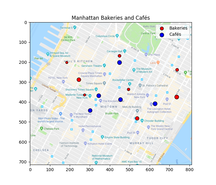
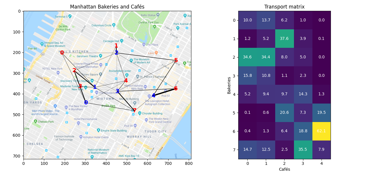
We will solve the Bakery/Cafés problem of transporting croissants from a number of Bakeries to Cafés in a City (in this case Manhattan). We did a quick google map search in Manhattan for bakeries and Cafés:

We extracted from this search their positions and generated fictional production and sale number (that both sum to the same value).

We have access to the position of Bakeries bakery_pos and their respective production bakery_prod which describe the source distribution. The Cafés where the croissants are sold are defined also by their position cafe_pos and cafe_prod, and describe the target distribution. For fun we also provide a map Imap that will illustrate the position of these shops in the city.

Now we load the data

data = np.load('../data/manhattan.npz')

bakery_pos = data['bakery_pos']
bakery_prod = data['bakery_prod']
cafe_pos = data['cafe_pos']
cafe_prod = data['cafe_prod']
Imap = data['Imap']

print('Bakery production: {}'.format(bakery_prod))
print('Cafe sale: {}'.format(cafe_prod))
print('Total croissants : {}'.format(cafe_prod.sum()))

Bakery production: [31. 48. 82. 30. 40. 48. 89. 73.]
Cafe sale: [82. 88. 92. 88. 91.]
Total croissants : 441.0

Plotting bakeries in the city

Next we plot the position of the bakeries and cafés on the map. The size of the circle is proportional to their production.

pl.figure(1, (7, 6))
pl.clf()
pl.imshow(Imap, interpolation='bilinear')  # plot the map
pl.scatter(bakery_pos[:, 0], bakery_pos[:, 1], s=bakery_prod, c='r', ec='k', label='Bakeries')
pl.scatter(cafe_pos[:, 0], cafe_pos[:, 1], s=cafe_prod, c='b', ec='k', label='Cafés')
pl.legend()
pl.title('Manhattan Bakeries and Cafés')

Text(0.5, 1.0, 'Manhattan Bakeries and Cafés')

Cost matrix

We can now compute the cost matrix between the bakeries and the cafés, which will be the transport cost matrix. This can be done using the ot.dist function that defaults to squared Euclidean distance but can return other things such as cityblock (or Manhattan distance).

C = ot.dist(bakery_pos, cafe_pos)

labels = [str(i) for i in range(len(bakery_prod))]
f = pl.figure(2, (14, 7))
pl.clf()
pl.subplot(121)
pl.imshow(Imap, interpolation='bilinear')  # plot the map
for i in range(len(cafe_pos)):
    pl.text(cafe_pos[i, 0], cafe_pos[i, 1], labels[i], color='b',
            fontsize=14, fontweight='bold', ha='center', va='center')
for i in range(len(bakery_pos)):
    pl.text(bakery_pos[i, 0], bakery_pos[i, 1], labels[i], color='r',
            fontsize=14, fontweight='bold', ha='center', va='center')
pl.title('Manhattan Bakeries and Cafés')

ax = pl.subplot(122)
im = pl.imshow(C, cmap="coolwarm")
pl.title('Cost matrix')
cbar = pl.colorbar(im, ax=ax, shrink=0.5, use_gridspec=True)
cbar.ax.set_ylabel("cost", rotation=-90, va="bottom")

pl.xlabel('Cafés')
pl.ylabel('Bakeries')
pl.tight_layout()

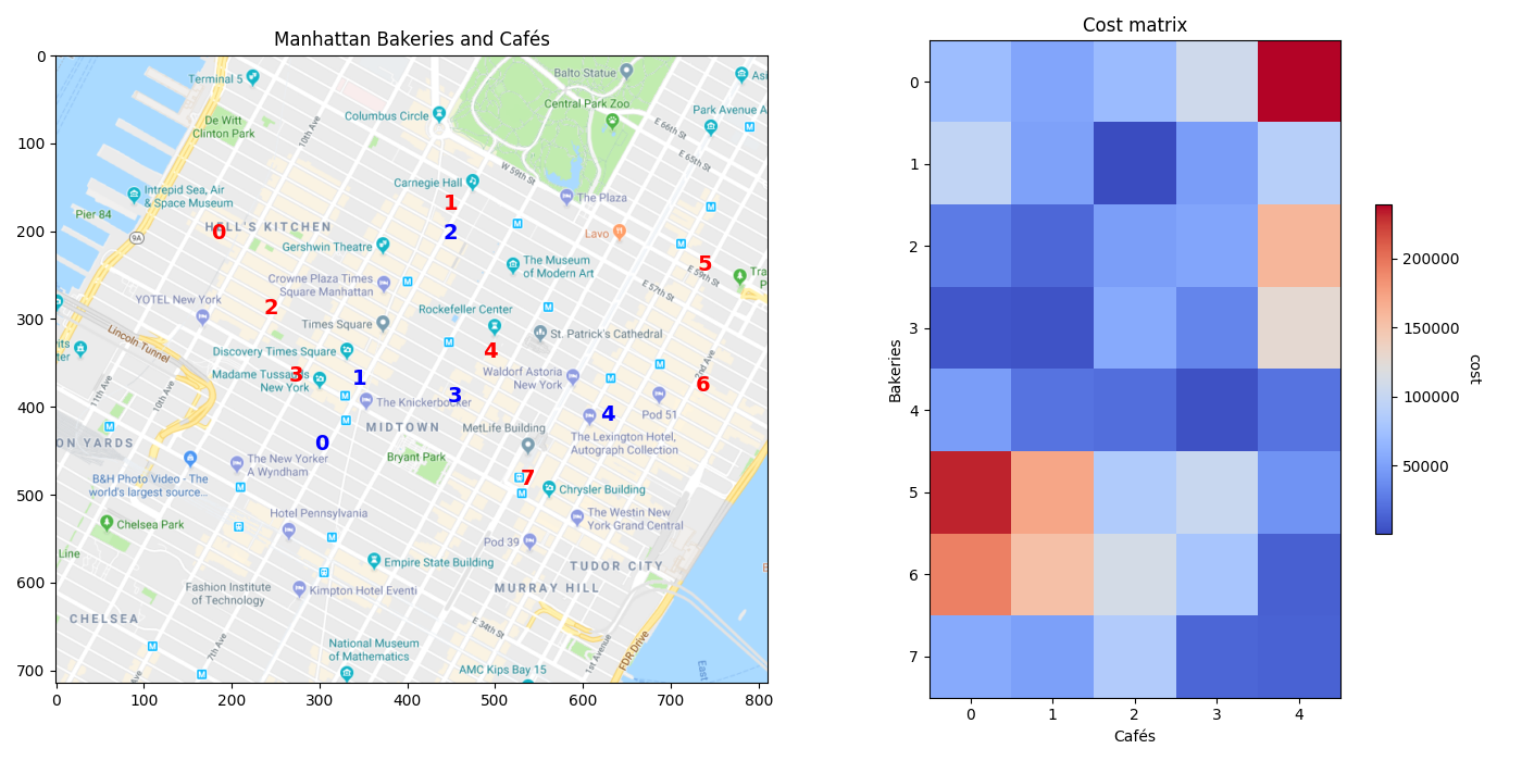
The red cells in the matrix image show the bakeries and cafés that are further away, and thus more costly to transport from one to the other, while the blue ones show those that are very close to each other, with respect to the squared Euclidean distance.

Solving the OT problem with ot.emd

start = time.time()
ot_emd = ot.emd(bakery_prod, cafe_prod, C)
time_emd = time.time() - start

The function returns the transport matrix, which we can then visualize (next section).

Transportation plan visualization

A good visualization of the OT matrix in the 2D plane is to denote the transportation of mass between a Bakery and a Café by a line. This can easily be done with a double for loop.

In order to make it more interpretable one can also use the alpha parameter of plot and set it to alpha=G[i,j]/G.max().

# Plot the matrix and the map
f = pl.figure(3, (14, 7))
pl.clf()
pl.subplot(121)
pl.imshow(Imap, interpolation='bilinear')  # plot the map
for i in range(len(bakery_pos)):
    for j in range(len(cafe_pos)):
        pl.plot([bakery_pos[i, 0], cafe_pos[j, 0]], [bakery_pos[i, 1], cafe_pos[j, 1]],
                '-k', lw=3. * ot_emd[i, j] / ot_emd.max())
for i in range(len(cafe_pos)):
    pl.text(cafe_pos[i, 0], cafe_pos[i, 1], labels[i], color='b', fontsize=14,
            fontweight='bold', ha='center', va='center')
for i in range(len(bakery_pos)):
    pl.text(bakery_pos[i, 0], bakery_pos[i, 1], labels[i], color='r', fontsize=14,
            fontweight='bold', ha='center', va='center')
pl.title('Manhattan Bakeries and Cafés')

ax = pl.subplot(122)
im = pl.imshow(ot_emd)
for i in range(len(bakery_prod)):
    for j in range(len(cafe_prod)):
        text = ax.text(j, i, '{0:g}'.format(ot_emd[i, j]),
                       ha="center", va="center", color="w")
pl.title('Transport matrix')

pl.xlabel('Cafés')
pl.ylabel('Bakeries')
pl.tight_layout()

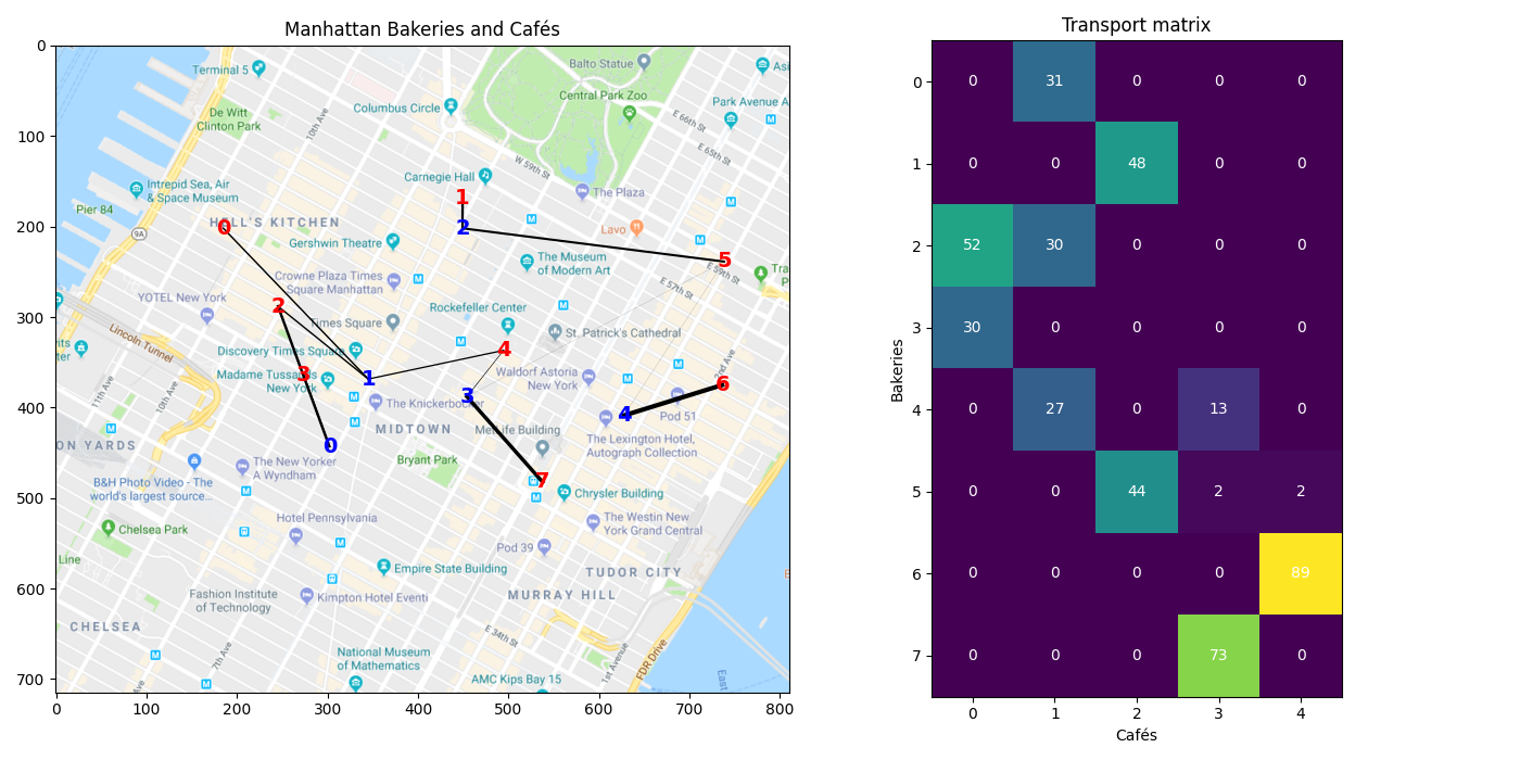
The transport matrix gives the number of croissants that can be transported from each bakery to each café. We can see that the bakeries only need to transport croissants to one or two cafés, the transport matrix being very sparse.

OT loss and dual variables

The resulting wasserstein loss loss is of the form:

\[W=\sum_{i,j}\gamma_{i,j}C_{i,j}\]

where \(\gamma\) is the optimal transport matrix.

W = np.sum(ot_emd * C)
print('Wasserstein loss (EMD) = {0:.2f}'.format(W))

Wasserstein loss (EMD) = 10838179.41

Regularized OT with Sinkhorn

The Sinkhorn algorithm is very simple to code. You can implement it directly using the following pseudo-code

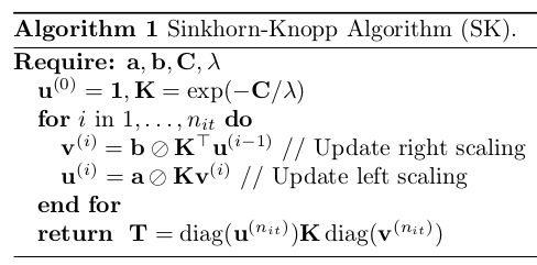
In this algorithm, \(\oslash\) corresponds to the element-wise division.

An alternative is to use the POT toolbox with ot.sinkhorn

Be careful of numerical problems. A good pre-processing for Sinkhorn is to divide the cost matrix C by its maximum value.

Algorithm

# Compute Sinkhorn transport matrix from algorithm
reg = 0.1
K = np.exp(-C / C.max() / reg)
nit = 100
u = np.ones((len(bakery_prod), ))
for i in range(1, nit):
    v = cafe_prod / np.dot(K.T, u)
    u = bakery_prod / (np.dot(K, v))
ot_sink_algo = np.atleast_2d(u).T * (K * v.T)  # Equivalent to np.dot(np.diag(u), np.dot(K, np.diag(v)))

# Compute Sinkhorn transport matrix with POT
ot_sinkhorn = ot.sinkhorn(bakery_prod, cafe_prod, reg=reg, M=C / C.max())

# Difference between the 2
print('Difference between algo and ot.sinkhorn = {0:.2g}'.format(np.sum(np.power(ot_sink_algo - ot_sinkhorn, 2))))

Difference between algo and ot.sinkhorn = 2.1e-20

Plot the matrix and the map

print('Min. of Sinkhorn\'s transport matrix = {0:.2g}'.format(np.min(ot_sinkhorn)))

f = pl.figure(4, (13, 6))
pl.clf()
pl.subplot(121)
pl.imshow(Imap, interpolation='bilinear')  # plot the map
for i in range(len(bakery_pos)):
    for j in range(len(cafe_pos)):
        pl.plot([bakery_pos[i, 0], cafe_pos[j, 0]],
                [bakery_pos[i, 1], cafe_pos[j, 1]],
                '-k', lw=3. * ot_sinkhorn[i, j] / ot_sinkhorn.max())
for i in range(len(cafe_pos)):
    pl.text(cafe_pos[i, 0], cafe_pos[i, 1], labels[i], color='b',
            fontsize=14, fontweight='bold', ha='center', va='center')
for i in range(len(bakery_pos)):
    pl.text(bakery_pos[i, 0], bakery_pos[i, 1], labels[i], color='r',
            fontsize=14, fontweight='bold', ha='center', va='center')
pl.title('Manhattan Bakeries and Cafés')

ax = pl.subplot(122)
im = pl.imshow(ot_sinkhorn)
for i in range(len(bakery_prod)):
    for j in range(len(cafe_prod)):
        text = ax.text(j, i, np.round(ot_sinkhorn[i, j], 1),
                       ha="center", va="center", color="w")
pl.title('Transport matrix')

pl.xlabel('Cafés')
pl.ylabel('Bakeries')
pl.tight_layout()

Min. of Sinkhorn's transport matrix = 0.0008

We notice right away that the matrix is not sparse at all with Sinkhorn, each bakery delivering croissants to all 5 cafés with that solution. Also, this solution gives a transport with fractions, which does not make sense in the case of croissants. This was not the case with EMD.

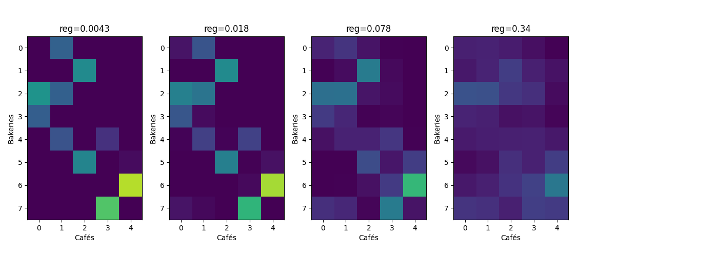
Varying the regularization parameter in Sinkhorn

reg_parameter = np.logspace(-3, 0, 20)
W_sinkhorn_reg = np.zeros((len(reg_parameter), ))
time_sinkhorn_reg = np.zeros((len(reg_parameter), ))

f = pl.figure(5, (14, 5))
pl.clf()
max_ot = 100  # plot matrices with the same colorbar
for k in range(len(reg_parameter)):
    start = time.time()
    ot_sinkhorn = ot.sinkhorn(bakery_prod, cafe_prod, reg=reg_parameter[k], M=C / C.max())
    time_sinkhorn_reg[k] = time.time() - start

    if k % 4 == 0 and k > 0:  # we only plot a few
        ax = pl.subplot(1, 5, k // 4)
        im = pl.imshow(ot_sinkhorn, vmin=0, vmax=max_ot)
        pl.title('reg={0:.2g}'.format(reg_parameter[k]))
        pl.xlabel('Cafés')
        pl.ylabel('Bakeries')

    # Compute the Wasserstein loss for Sinkhorn, and compare with EMD
    W_sinkhorn_reg[k] = np.sum(ot_sinkhorn * C)
pl.tight_layout()

/home/circleci/project/ot/bregman/_sinkhorn.py:531: UserWarning: Sinkhorn did not converge. You might want to increase the number of iterations `numItermax` or the regularization parameter `reg`.
  warnings.warn("Sinkhorn did not converge. You might want to "

This series of graph shows that the solution of Sinkhorn starts with something very similar to EMD (although not sparse) for very small values of the regularization parameter, and tends to a more uniform solution as the regularization parameter increases.

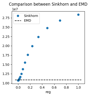
Wasserstein loss and computational time

# Plot the matrix and the map
f = pl.figure(6, (4, 4))
pl.clf()
pl.title("Comparison between Sinkhorn and EMD")

pl.plot(reg_parameter, W_sinkhorn_reg, 'o', label="Sinkhorn")
XLim = pl.xlim()
pl.plot(XLim, [W, W], '--k', label="EMD")
pl.legend()
pl.xlabel("reg")
pl.ylabel("Wasserstein loss")

Text(3.972222222222223, 0.5, 'Wasserstein loss')

In this last graph, we show the impact of the regularization parameter on the Wasserstein loss. We can see that higher values of reg leads to a much higher Wasserstein loss.

The Wasserstein loss of EMD is displayed for comparison. The Wasserstein loss of Sinkhorn can be a little lower than that of EMD for low values of reg, but it quickly gets much higher.