ot.utils
Various useful functions
Functions
- ot.utils.apply_scaler(X_s, X_t, scaler=None)[source]
Apply a scaler to two arrays.
Dispatches based on the type of
scaler:None: returns inputs unchanged.Object with a
.transform()method : callsscaler.transform()on each.Callable : calls
scaler()on each (covers functions, lambdas, PyTorch transforms, neural network encoders, etc.).
- Parameters:
X_s (array-like) – Source samples.
X_t (array-like) – Target samples.
scaler (None, object with .transform(), or callable, optional) – Preprocessing to apply.
- Returns:
X_s_out (array-like) – Possibly transformed source samples.
X_t_out (array-like) – Possibly transformed target samples.
- ot.utils.check_number_threads(numThreads)[source]
Checks whether or not the requested number of threads has a valid value.
- ot.utils.check_random_state(seed)[source]
Turn seed into a np.random.RandomState instance
- Parameters:
seed (None | int | instance of RandomState) – If seed is None, return the RandomState singleton used by np.random. If seed is an int, return a new RandomState instance seeded with seed. If seed is already a RandomState instance, return it. Otherwise raise ValueError.
- ot.utils.clean_zeros(a, b, M)[source]
Remove all components with zeros weights in \(\mathbf{a}\) and \(\mathbf{b}\)
- ot.utils.cost_normalization(C, norm=None, return_value=False, value=None)[source]
Apply normalization to the loss matrix
- Parameters:
C (ndarray, shape (n1, n2)) – The cost matrix to normalize.
norm (str) – Type of normalization from ‘median’, ‘max’, ‘log’, ‘loglog’. Any other value do not normalize.
- Returns:
C – The input cost matrix normalized according to given norm.
- Return type:
ndarray, shape (n1, n2)
- ot.utils.dist(x1, x2=None, metric='sqeuclidean', p=2, w=None, backend='auto', nx=None, use_tensor=False)[source]
Compute distance between samples in \(\mathbf{x_1}\) and \(\mathbf{x_2}\)
Note
This function is backend-compatible and will work on arrays from all compatible backends for the following metrics: ‘sqeuclidean’, ‘euclidean’, ‘cityblock’, ‘minkowski’, ‘cosine’, ‘correlation’.
- Parameters:
x1 (array-like, shape (n1,d)) – matrix with n1 samples of size d
x2 (array-like, shape (n2,d), optional) – matrix with n2 samples of size d (if None then \(\mathbf{x_2} = \mathbf{x_1}\))
metric (str | callable, optional) – ‘sqeuclidean’ or ‘euclidean’ on all backends. On numpy the function also accepts from the scipy.spatial.distance.cdist function : ‘braycurtis’, ‘canberra’, ‘chebyshev’, ‘cityblock’, ‘correlation’, ‘cosine’, ‘dice’, ‘euclidean’, ‘hamming’, ‘jaccard’, ‘kulczynski1’, ‘mahalanobis’, ‘matching’, ‘minkowski’, ‘rogerstanimoto’, ‘russellrao’, ‘seuclidean’, ‘sokalmichener’, ‘sokalsneath’, ‘sqeuclidean’, ‘wminkowski’, ‘yule’.
p (float, optional) – p-norm for the Minkowski and the Weighted Minkowski metrics. Default value is 2.
w (array-like, rank 1) – Weights for the weighted metrics.
backend (str, optional) – Backend to use for the computation. If ‘auto’, the backend is automatically selected based on the input data. if ‘scipy’, the
scipy.spatial.distance.cdistfunction is used (and gradients are detached).use_tensor (bool, optional) – If true use tensorized computation for the distance matrix which can cause memory issues for large datasets. Default is False and the parameter is used only for the ‘cityblock’ and ‘minkowski’ metrics.
nx (Backend, optional) – Backend to perform computations on. If omitted, the backend defaults to that of x1.
- Returns:
M – distance matrix computed with given metric
- Return type:
array-like, shape (n1, n2)
- ot.utils.dist0(n, method='lin_square')[source]
Compute standard cost matrices of size (n, n) for OT problems
Examples using ot.utils.dist0
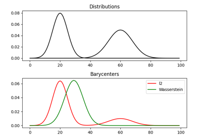
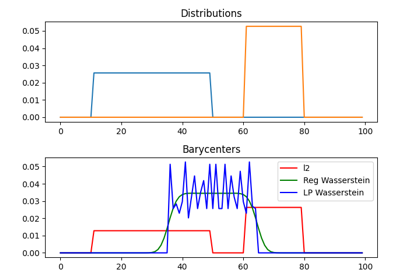
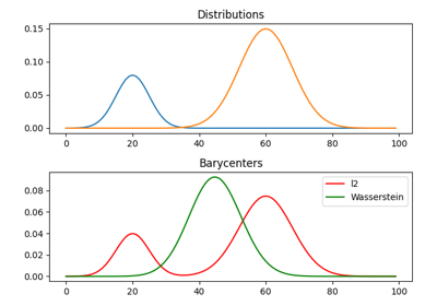
1D Wasserstein barycenter: exact LP vs entropic regularization
1D Wasserstein barycenter demo for Unbalanced distributions
- ot.utils.euclidean_distances(X, Y, squared=False, nx=None)[source]
Considering the rows of \(\mathbf{X}\) (and \(\mathbf{Y} = \mathbf{X}\)) as vectors, compute the distance matrix between each pair of vectors.
Note
This function is backend-compatible and will work on arrays from all compatible backends.
- Parameters:
X (array-like, shape (n_samples_1, n_features))
Y (array-like, shape (n_samples_2, n_features))
squared (boolean, optional) – Return squared Euclidean distances.
- Returns:
distances
- Return type:
array-like, shape (n_samples_1, n_samples_2)
- ot.utils.exp_bures(Sigma, S, nx=None)[source]
Exponential map in Bures-Wasserstein space at Sigma:
\[\exp_\Sigma(S) = (I_d+S)\Sigma(I_d+S).\]- Parameters:
Sigma (array-like (d,d)) – SPD matrix
S (array-like (d,d)) – Symmetric matrix
nx (module, optional) – The numerical backend module to use. If not provided, the backend will be fetched from the input matrices Sigma, S.
- Returns:
P – SPD matrix obtained as the exponential map of S at Sigma
- Return type:
array-like (d,d)
- ot.utils.fun_to_numpy(fun, arr, nx, warn=True)[source]
Convert a function to a numpy function.
- Parameters:
- Returns:
fun_numpy – The converted function.
- Return type:
callable
- ot.utils.get_coordinate_circle(x)[source]
For \(x\in S^1 \subset \mathbb{R}^2\), returns the coordinates in turn (in [0,1[).
\[u = \frac{\pi + \mathrm{atan2}(-x_2,-x_1)}{2\pi}\]- Parameters:
x (ndarray, shape (n, 2)) – Samples on the circle with ambient coordinates
- Returns:
x_t – Coordinates on [0,1[
- Return type:
ndarray, shape (n,)
Examples
>>> u = np.array([[0.2,0.5,0.8]]) * (2 * np.pi)
>>> x1, y1 = np.cos(u), np.sin(u)
>>> x = np.concatenate([x1, y1]).T
>>> get_coordinate_circle(x)
array([0.2, 0.5, 0.8])
- ot.utils.get_lowrank_lazytensor(Q, R, d=None, nx=None)[source]
Get a low rank LazyTensor T=Q@R^T or T=Q@diag(d)@R^T
- Parameters:
Q (ndarray, shape (n, r)) – First factor of the lowrank tensor
R (ndarray, shape (m, r)) – Second factor of the lowrank tensor
d (ndarray, shape (r,), optional) – Diagonal of the lowrank tensor
nx (Backend, optional) – Backend to use for the reduction
- Returns:
T – Lowrank tensor T=Q@R^T or T=Q@diag(d)@R^T
- Return type:
- ot.utils.get_parameter_pair(parameter)[source]
Extract a pair of parameters from a given parameter Used in unbalanced OT and COOT solvers to handle marginal regularization and entropic regularization.
- Parameters:
parameter (float or indexable object)
nx (backend object)
- Returns:
param_1 (float)
param_2 (float)
- ot.utils.label_normalization(y, start=0, nx=None)[source]
Transform labels to start at a given value
- Parameters:
- Returns:
y – The input vector of labels normalized according to given start value.
- Return type:
array-like, shape (n1, )
- ot.utils.labels_to_masks(y, type_as=None, nx=None)[source]
Transforms (n_samples,) vector of labels into a (n_samples, n_labels) matrix of masks.
- Parameters:
y (array-like, shape (n_samples, )) – The vector of labels.
type_as (array_like) – Array of the same type of the expected output.
nx (Backend, optional) – Backend to perform computations on. If omitted, the backend defaults to that of y.
- Returns:
masks – The (n_samples, n_labels) matrix of label masks.
- Return type:
array-like, shape (n_samples, n_labels)
- ot.utils.parmap(f, X, nprocs='default')[source]
parallel map for multiprocessing. The function has been deprecated and only performs a regular map.
- ot.utils.proj_SDP(S, nx=None, vmin=0.0)[source]
Project a symmetric matrix onto the space of symmetric matrices with eigenvalues larger or equal to vmin.
- Parameters:
S (array_like (n, d, d) or (d, d)) – The input symmetric matrix or matrices.
nx (module, optional) – The numerical backend module to use. If not provided, the backend will be fetched from the input matrix S.
vmin (float, optional) – The minimum value for the eigenvalues. Eigenvalues below this value will be clipped to vmin.
note: (..) – This function is backend-compatible and will work on arrays: from all compatible backends.
- Returns:
P – The projected symmetric positive definite matrix.
- Return type:
ndarray (n, d, d) or (d, d)
Examples using ot.utils.proj_SDP
- ot.utils.proj_simplex(v, z=1)[source]
Compute the closest point (orthogonal projection) on the generalized (n-1)-simplex of a vector \(\mathbf{v}\) wrt. to the Euclidean distance, thus solving:
\[ \begin{align}\begin{aligned}\mathcal{P}(w) \in \mathop{\arg \min}_\gamma \| \gamma - \mathbf{v} \|_2\\s.t. \ \gamma^T \mathbf{1} = z\\ \gamma \geq 0\end{aligned}\end{align} \]If \(\mathbf{v}\) is a 2d array, compute all the projections wrt. axis 0
Note
This function is backend-compatible and will work on arrays from all compatible backends.
- Parameters:
v ({array-like}, shape (n, d))
z (int, optional) – ‘size’ of the simplex (each vectors sum to z, 1 by default)
- Returns:
h – Array of projections on the simplex
- Return type:
ndarray, shape (n, d)
Examples using ot.utils.proj_simplex
Optimizing the Gromov-Wasserstein distance with PyTorch
- ot.utils.projection_sparse_simplex(V, max_nz, z=1, axis=None, nx=None)[source]
Projection of \(\mathbf{V}\) onto the simplex with cardinality constraint (maximum number of non-zero elements) and then scaled by z.
\[\begin{split}P\left(\mathbf{V}, \text{max_nz}, z\right) = \mathop{\arg \min}_{\substack{\mathbf{y} >= 0 \\ \sum_i \mathbf{y}_i = z} \\ ||p||_0 \le \text{max_nz}} \quad \|\mathbf{y} - \mathbf{V}\|^2\end{split}\]- Parameters:
V (1-dim or 2-dim ndarray)
max_nz (int) – Maximum number of non-zero elements in the projection. If max_nz is larger than the number of elements in V, then the projection is equivalent to proj_simplex(V, z).
z (float or array) – If array, len(z) must be compatible with \(\mathbf{V}\)
axis (None or int) –
axis=None: project \(\mathbf{V}\) by \(P(\mathbf{V}.\mathrm{ravel}(), \text{max_nz}, z)\)
axis=1: project each \(\mathbf{V}_i\) by \(P(\mathbf{V}_i, \text{max_nz}, z_i)\)
axis=0: project each \(\mathbf{V}_{:, j}\) by \(P(\mathbf{V}_{:, j}, \text{max_nz}, z_j)\)
- Returns:
projection
- Return type:
ndarray, shape \(\mathbf{V}\).shape
References
- ot.utils.reduce_lazytensor(a, func, axis=None, nx=None, batch_size=100)[source]
Reduce a LazyTensor along an axis with function fun using batches.
When axis=None, reduce the LazyTensor to a scalar as a sum of fun over batches taken along dim.
Warning
This function works for tensor of any order but the reduction can be done only along the first two axis (or global). Also, in order to work, it requires that the slice of size batch_size along the axis to reduce (or axis 0 if axis=None) is can be computed and fits in memory.
- Parameters:
a (LazyTensor) – LazyTensor to reduce
func (callable) – Function to apply to the LazyTensor
axis (int, optional) – Axis along which to reduce the LazyTensor. If None, reduce the LazyTensor to a scalar as a sum of fun over batches taken along axis 0. If 0 or 1 reduce the LazyTensor to a vector/matrix as a sum of fun over batches taken along axis.
nx (Backend, optional) – Backend to use for the reduction
batch_size (int, optional) – Size of the batches to use for the reduction (default=100)
- Returns:
res – Result of the reduction
- Return type:
array-like
- ot.utils.sparse_ot_dist(x1, x2, i, j, w=None, metric='sqeuclidean', p=2, batch_size=None)[source]
Compute ot distance between samples in \(\mathbf{x_1}\) and \(\mathbf{x_2}\) with sparse weights given by w for the pairs of samples with indices i and j.
Note
This function is backend-compatible and will work on arrays from all compatible backends for the following metrics: ‘sqeuclidean’, ‘euclidean’, ‘cityblock’, ‘minkowski’.
- Parameters:
x1 (array-like, shape (n1,d)) – matrix with n1 samples of size d
x2 (array-like, shape (n2,d), optional) – matrix with n2 samples of size d (if None then \(\mathbf{x_2} = \mathbf{x_1}\))
i (array-like, shape (k,)) – indices of samples in x1 to compute distance from
j (array-like, shape (k,)) – indices of samples in x2 to compute distance to
w (array-like, shape (k,), optional) – weights for each pair of samples to compute distance between. If None, all pairs are weighted equally (=1/k).
metric (str | callable, optional) – ‘sqeuclidean’, ‘euclidean’, ‘cityblock’ or ‘minkowski’.
p (float, optional) – p-norm for the Minkowski metric. Default value is 2.
batch_size (int, optional) – If specified, compute the distance in batches of size batch_size to avoid memory issues for large datasets. Default is None (no batching).
- Returns:
dist – sum of the distance between \(\mathbf{x_1}_i\) and \(\mathbf{x_2}_j\) computed with given metric and weighted by w
- Return type:
- ot.utils.split_sample_ratio(X_a, a=None, ratio=0.5, random_split=False, random_state=None, nx=None)[source]
Split distribution according to a ratio of weights (using point ordering).
- Parameters:
X_a (array-like, shape (n_samples_a, dim)) – samples in the source domain
a (array-like, shape (dim_a,), optional) – Samples weights in the source domain (default is uniform)
nx (backend, optional) – Backend for array operations, by default None (auto-detect)
ratio (float, optional) – Ratio of the split, by default 0.5
random_split (bool, optional) – Whether to split randomly, by default False
random_state (int, optional) – Random state for reproducibility, by default None
- Returns:
X_a1 (array-like, shape (n_samples_a1, dim)) – First half of the samples in the source domain
X_a2 (array-like, shape (n_samples_a2, dim)) – Second half of the samples in the source domain
a1 (array-like, shape (dim_a1,)) – First half of the weights in the source domain
a2 (array-like, shape (dim_a2,)) – Second half of the weights in the source domain
sel_a1 (slice, ndarray-like) – Slice or indexes for the first half of the samples in the source domain
sel_a2 (slice, ndarray-like) – Slice or indexes for the second half of the samples in the source domain
- ot.utils.unif(n, type_as=None)[source]
Return a uniform histogram of length n (simplex).
- Parameters:
n (int) – number of bins in the histogram
type_as (array-like) – array of the same type of the expected output (numpy/pytorch/jax)
- Returns:
h – histogram of length n such that \(\forall i, \mathbf{h}_i = \frac{1}{n}\)
- Return type:
array-like, shape (n,)
Classes
- class ot.utils.BaryResult(X=None, C=None, b=None, value=None, value_linear=None, value_quad=None, log=None, list_res=None, status=None, backend=None)[source]
Base class for OT barycenter results.
- Parameters:
X (array-like, shape (n, d)) – Barycenter features.
C (array-like, shape (n, n)) – Barycenter structure for Gromov Wasserstein solutions.
b (array-like, shape (n,)) – Barycenter weights.
value (float, array-like) – Full transport cost, including possible regularization terms and quadratic term for Gromov Wasserstein solutions.
value_linear (float, array-like) – The linear part of the transport cost, i.e. the product between the transport plan and the cost.
value_quad (float, array-like) – The quadratic part of the transport cost for Gromov-Wasserstein solutions.
log (dict) – Dictionary containing potential information about the solver.
list_res (list of OTResult) – List of results for the individual OT matching with input distributions considered as sources and the learned barycenter distribution as target.
- X
Barycenter features.
- Type:
array-like, shape (n, d)
- C
Barycenter structure for Gromov Wasserstein solutions.
- Type:
array-like, shape (n, n)
- b
Barycenter weights.
- Type:
array-like, shape (n,)
- value
Full transport cost, including possible regularization terms and quadratic term for Gromov Wasserstein solutions.
- Type:
float, array-like
- value_linear
The linear part of the transport cost, i.e. the product between the transport plan and the cost.
- Type:
float, array-like
- value_quad
The quadratic part of the transport cost for Gromov-Wasserstein solutions.
- Type:
float, array-like
- property C
Barycenter structure for Gromov Wasserstein solutions.
- property X
Barycenter features.
- property b
Barycenter weights.
- property citation
Appropriate citation(s) for this result, in plain text and BibTex formats.
- property list_res
List of results for the individual OT matching.
- property log
Dictionary containing potential information about the solver.
- property status
Optimization status of the solver.
- property value
Full transport cost, including possible regularization terms and quadratic term for Gromov Wasserstein solutions.
- property value_linear
The “minimal” transport cost, i.e. the product between the transport plan and the cost.
- property value_quad
The quadratic part of the transport cost for Gromov-Wasserstein solutions.
Examples using ot.utils.BaryResult
- class ot.utils.BaseEstimator[source]
Base class for most objects in POT
Code adapted from sklearn BaseEstimator class
Notes
All estimators should specify all the parameters that can be set at the class level in their
__init__as explicit keyword arguments (no*argsor**kwargs).- get_params(deep=True)[source]
Get parameters for this estimator.
- Parameters:
deep (bool, optional) – If True, will return the parameters for this estimator and contained subobjects that are estimators.
- Returns:
params – Parameter names mapped to their values.
- Return type:
mapping of string to any
- set_params(**params)[source]
Set the parameters of this estimator.
The method works on simple estimators as well as on nested objects (such as pipelines). The latter have parameters of the form
<component>__<parameter>so that it’s possible to update each component of a nested object.- Return type:
self
Examples using ot.utils.BaseEstimator
OT with Laplacian regularization for domain adaptation
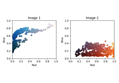
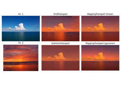
OT for image color adaptation with mapping estimation
OT for domain adaptation on empirical distributions
- class ot.utils.DataScaler(norm='standard')[source]
Backend-aware data scaler with sklearn-compatible API.
Fit normalization statistics on a single array or on the concatenation of multiple arrays (joint fitting), then apply the same fixed transform to any array. Supports NumPy, PyTorch, JAX, and TensorFlow backends via POT’s backend abstraction.
- Parameters:
norm (str, optional) –
Normalization method. One of:
'standard'(default) : zero mean, unit variance per feature'minmax': scale each feature to [0, 1]'l2': unit L2-norm per sample (row-wise, stateless)
- mean_
Per-feature means (only for
norm='standard').- Type:
array-like
- std_
Per-feature standard deviations (only for
norm='standard').- Type:
array-like
- min_
Per-feature minimums (only for
norm='minmax').- Type:
array-like
- max_
Per-feature maximums (only for
norm='minmax').- Type:
array-like
Examples
>>> import numpy as np
>>> from ot.utils import DataScaler
>>> X_s = np.array([[1.0, 100.0], [2.0, 200.0]])
>>> X_t = np.array([[3.0, 300.0], [4.0, 400.0]])
>>> scaler = DataScaler(norm='standard').fit([X_s, X_t])
>>> X_s_scaled = scaler.transform(X_s)
- fit(X)[source]
Compute normalization statistics from one array or a list of arrays.
When given a list, arrays are concatenated along axis 0 before computing statistics (joint fitting).
- Parameters:
X (array-like or list of array-like) – Data to fit on. If a list, arrays must have the same number of features (columns).
- Returns:
self
- Return type:
- transform(X)[source]
Apply the fitted transformation to X.
- Parameters:
X (array-like or list of array-like) – Data to transform. If a list, each element is transformed and returned as a list.
- Returns:
X_scaled – Transformed data, same shape and backend as X. If X was a list, returns a list of transformed arrays.
- Return type:
array-like or list of array-like
Examples using ot.utils.DataScaler
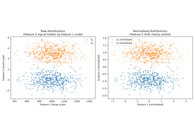
Sliced Wasserstein Distance with input scaling (DataScaler)
- class ot.utils.LazyTensor(shape, getitem, **kwargs)[source]
A lazy tensor is a tensor that is not stored in memory. Instead, it is defined by a function that computes its values on the fly from slices.
- Parameters:
Examples
>>> import numpy as np
>>> v = np.arange(5)
>>> def getitem(i,j, v):
...     return v[i,None]+v[None,j]
>>> T = LazyTensor((5,5),getitem, v=v)
>>> T[1,2]
array([3])
>>> T[1,:]
array([[1, 2, 3, 4, 5]])
>>> T[:]
array([[0, 1, 2, 3, 4],
       [1, 2, 3, 4, 5],
       [2, 3, 4, 5, 6],
       [3, 4, 5, 6, 7],
       [4, 5, 6, 7, 8]])
Examples using ot.utils.LazyTensor
- class ot.utils.OTResult(potentials=None, value=None, value_linear=None, value_quad=None, plan=None, log=None, backend=None, sparse_plan=None, lazy_plan=None, status=None, batch_size=100)[source]
Base class for OT results.
- Parameters:
potentials (tuple of array-like, shape (n1, n2)) – Dual potentials, i.e. Lagrange multipliers for the marginal constraints. This pair of arrays has the same shape, numerical type and properties as the input weights “a” and “b”.
value (float, array-like) – Full transport cost, including possible regularization terms and quadratic term for Gromov Wasserstein solutions.
value_linear (float, array-like) – The linear part of the transport cost, i.e. the product between the transport plan and the cost.
value_quad (float, array-like) – The quadratic part of the transport cost for Gromov-Wasserstein solutions.
plan (array-like, shape (n1, n2)) – Transport plan, encoded as a dense array.
log (dict) – Dictionary containing potential information about the solver.
backend (Backend) – Backend used to compute the results.
sparse_plan (array-like, shape (n1, n2)) – Transport plan, encoded as a sparse array.
lazy_plan (LazyTensor) – Transport plan, encoded as a symbolic POT or KeOps LazyTensor.
batch_size (int) – Batch size used to compute the results/marginals for LazyTensor.
- potentials
Dual potentials, i.e. Lagrange multipliers for the marginal constraints. This pair of arrays has the same shape, numerical type and properties as the input weights “a” and “b”.
- Type:
tuple of array-like, shape (n1, n2)
- potential_a
First dual potential, associated to the “source” measure “a”.
- Type:
array-like, shape (n1,)
- potential_b
Second dual potential, associated to the “target” measure “b”.
- Type:
array-like, shape (n2,)
- value
Full transport cost, including possible regularization terms and quadratic term for Gromov Wasserstein solutions.
- Type:
float, array-like
- value_linear
The linear part of the transport cost, i.e. the product between the transport plan and the cost.
- Type:
float, array-like
- value_quad
The quadratic part of the transport cost for Gromov-Wasserstein solutions.
- Type:
float, array-like
- plan
Transport plan, encoded as a dense array.
- Type:
array-like, shape (n1, n2)
- sparse_plan
Transport plan, encoded as a sparse array.
- Type:
array-like, shape (n1, n2)
- lazy_plan
Transport plan, encoded as a symbolic POT or KeOps LazyTensor.
- Type:
- marginals
Marginals of the transport plan: should be very close to “a” and “b” for balanced OT.
- Type:
tuple of array-like, shape (n1,), (n2,)
- marginal_a
Marginal of the transport plan for the “source” measure “a”.
- Type:
array-like, shape (n1,)
- marginal_b
Marginal of the transport plan for the “target” measure “b”.
- Type:
array-like, shape (n2,)
- property a_to_b
Displacement vectors from the first to the second measure.
- property b_to_a
Displacement vectors from the second to the first measure.
- property citation
Appropriate citation(s) for this result, in plain text and BibTex formats.
- property lazy_plan
Transport plan, encoded as a symbolic KeOps LazyTensor.
- property log
Dictionary containing potential information about the solver.
- property marginal_a
First marginal of the transport plan, with the same shape as “a”.
- property marginal_b
Second marginal of the transport plan, with the same shape as “b”.
- property marginals
should be very close to “a” and “b” for balanced OT.
- Type:
Marginals of the transport plan
- property plan
Transport plan, encoded as a dense array.
- property potential_a
First dual potential, associated to the “source” measure “a”.
- property potential_b
Second dual potential, associated to the “target” measure “b”.
- property potentials
Dual potentials, i.e. Lagrange multipliers for the marginal constraints.
This pair of arrays has the same shape, numerical type and properties as the input weights “a” and “b”.
- property sparse_plan
Transport plan, encoded as a sparse array.
- property status
Optimization status of the solver.
- property value
Full transport cost, including possible regularization terms and quadratic term for Gromov Wasserstein solutions.
- property value_linear
The “minimal” transport cost, i.e. the product between the transport plan and the cost.
- property value_quad
The quadratic part of the transport cost for Gromov-Wasserstein solutions.
Examples using ot.utils.OTResult
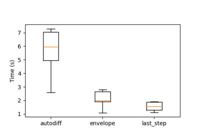
Different gradient computations for regularized optimal transport

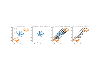
Solving Many Optimal Transport Problems in Parallel
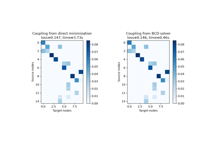
Solve Fused Unbalanced Gromov Wasserstein with Adam
- class ot.utils.deprecated(extra='')[source]
Decorator to mark a function or class as deprecated.
deprecated class from scikit-learn package https://github.com/scikit-learn/scikit-learn/blob/master/sklearn/utils/deprecation.py Issue a warning when the function is called/the class is instantiated and adds a warning to the docstring. The optional extra argument will be appended to the deprecation message and the docstring.
Note
To use this with the default value for extra, use empty parentheses:
>>> from ot.deprecation import deprecated
>>> @deprecated()
... def some_function(): pass
- Parameters:
extra (str) – To be added to the deprecation messages.
Exceptions
Aim at raising an Exception when a undefined parameter is called |
- class ot.utils.BaryResult(X=None, C=None, b=None, value=None, value_linear=None, value_quad=None, log=None, list_res=None, status=None, backend=None)[source]
Base class for OT barycenter results.
- Parameters:
X (array-like, shape (n, d)) – Barycenter features.
C (array-like, shape (n, n)) – Barycenter structure for Gromov Wasserstein solutions.
b (array-like, shape (n,)) – Barycenter weights.
value (float, array-like) – Full transport cost, including possible regularization terms and quadratic term for Gromov Wasserstein solutions.
value_linear (float, array-like) – The linear part of the transport cost, i.e. the product between the transport plan and the cost.
value_quad (float, array-like) – The quadratic part of the transport cost for Gromov-Wasserstein solutions.
log (dict) – Dictionary containing potential information about the solver.
list_res (list of OTResult) – List of results for the individual OT matching with input distributions considered as sources and the learned barycenter distribution as target.
- X
Barycenter features.
- Type:
array-like, shape (n, d)
- C
Barycenter structure for Gromov Wasserstein solutions.
- Type:
array-like, shape (n, n)
- b
Barycenter weights.
- Type:
array-like, shape (n,)
- value
Full transport cost, including possible regularization terms and quadratic term for Gromov Wasserstein solutions.
- Type:
float, array-like
- value_linear
The linear part of the transport cost, i.e. the product between the transport plan and the cost.
- Type:
float, array-like
- value_quad
The quadratic part of the transport cost for Gromov-Wasserstein solutions.
- Type:
float, array-like
- property C
Barycenter structure for Gromov Wasserstein solutions.
- property X
Barycenter features.
- property b
Barycenter weights.
- property citation
Appropriate citation(s) for this result, in plain text and BibTex formats.
- property list_res
List of results for the individual OT matching.
- property log
Dictionary containing potential information about the solver.
- property status
Optimization status of the solver.
- property value
Full transport cost, including possible regularization terms and quadratic term for Gromov Wasserstein solutions.
- property value_linear
The “minimal” transport cost, i.e. the product between the transport plan and the cost.
- property value_quad
The quadratic part of the transport cost for Gromov-Wasserstein solutions.
- class ot.utils.BaseEstimator[source]
Base class for most objects in POT
Code adapted from sklearn BaseEstimator class
Notes
All estimators should specify all the parameters that can be set at the class level in their
__init__as explicit keyword arguments (no*argsor**kwargs).- get_params(deep=True)[source]
Get parameters for this estimator.
- Parameters:
deep (bool, optional) – If True, will return the parameters for this estimator and contained subobjects that are estimators.
- Returns:
params – Parameter names mapped to their values.
- Return type:
mapping of string to any
- set_params(**params)[source]
Set the parameters of this estimator.
The method works on simple estimators as well as on nested objects (such as pipelines). The latter have parameters of the form
<component>__<parameter>so that it’s possible to update each component of a nested object.- Return type:
self
- class ot.utils.DataScaler(norm='standard')[source]
Backend-aware data scaler with sklearn-compatible API.
Fit normalization statistics on a single array or on the concatenation of multiple arrays (joint fitting), then apply the same fixed transform to any array. Supports NumPy, PyTorch, JAX, and TensorFlow backends via POT’s backend abstraction.
- Parameters:
norm (str, optional) –
Normalization method. One of:
'standard'(default) : zero mean, unit variance per feature'minmax': scale each feature to [0, 1]'l2': unit L2-norm per sample (row-wise, stateless)
- mean_
Per-feature means (only for
norm='standard').- Type:
array-like
- std_
Per-feature standard deviations (only for
norm='standard').- Type:
array-like
- min_
Per-feature minimums (only for
norm='minmax').- Type:
array-like
- max_
Per-feature maximums (only for
norm='minmax').- Type:
array-like
Examples
>>> import numpy as np
>>> from ot.utils import DataScaler
>>> X_s = np.array([[1.0, 100.0], [2.0, 200.0]])
>>> X_t = np.array([[3.0, 300.0], [4.0, 400.0]])
>>> scaler = DataScaler(norm='standard').fit([X_s, X_t])
>>> X_s_scaled = scaler.transform(X_s)
- fit(X)[source]
Compute normalization statistics from one array or a list of arrays.
When given a list, arrays are concatenated along axis 0 before computing statistics (joint fitting).
- Parameters:
X (array-like or list of array-like) – Data to fit on. If a list, arrays must have the same number of features (columns).
- Returns:
self
- Return type:
- transform(X)[source]
Apply the fitted transformation to X.
- Parameters:
X (array-like or list of array-like) – Data to transform. If a list, each element is transformed and returned as a list.
- Returns:
X_scaled – Transformed data, same shape and backend as X. If X was a list, returns a list of transformed arrays.
- Return type:
array-like or list of array-like
- class ot.utils.LazyTensor(shape, getitem, **kwargs)[source]
A lazy tensor is a tensor that is not stored in memory. Instead, it is defined by a function that computes its values on the fly from slices.
- Parameters:
Examples
>>> import numpy as np
>>> v = np.arange(5)
>>> def getitem(i,j, v):
...     return v[i,None]+v[None,j]
>>> T = LazyTensor((5,5),getitem, v=v)
>>> T[1,2]
array([3])
>>> T[1,:]
array([[1, 2, 3, 4, 5]])
>>> T[:]
array([[0, 1, 2, 3, 4],
       [1, 2, 3, 4, 5],
       [2, 3, 4, 5, 6],
       [3, 4, 5, 6, 7],
       [4, 5, 6, 7, 8]])
- class ot.utils.OTResult(potentials=None, value=None, value_linear=None, value_quad=None, plan=None, log=None, backend=None, sparse_plan=None, lazy_plan=None, status=None, batch_size=100)[source]
Base class for OT results.
- Parameters:
potentials (tuple of array-like, shape (n1, n2)) – Dual potentials, i.e. Lagrange multipliers for the marginal constraints. This pair of arrays has the same shape, numerical type and properties as the input weights “a” and “b”.
value (float, array-like) – Full transport cost, including possible regularization terms and quadratic term for Gromov Wasserstein solutions.
value_linear (float, array-like) – The linear part of the transport cost, i.e. the product between the transport plan and the cost.
value_quad (float, array-like) – The quadratic part of the transport cost for Gromov-Wasserstein solutions.
plan (array-like, shape (n1, n2)) – Transport plan, encoded as a dense array.
log (dict) – Dictionary containing potential information about the solver.
backend (Backend) – Backend used to compute the results.
sparse_plan (array-like, shape (n1, n2)) – Transport plan, encoded as a sparse array.
lazy_plan (LazyTensor) – Transport plan, encoded as a symbolic POT or KeOps LazyTensor.
batch_size (int) – Batch size used to compute the results/marginals for LazyTensor.
- potentials
Dual potentials, i.e. Lagrange multipliers for the marginal constraints. This pair of arrays has the same shape, numerical type and properties as the input weights “a” and “b”.
- Type:
tuple of array-like, shape (n1, n2)
- potential_a
First dual potential, associated to the “source” measure “a”.
- Type:
array-like, shape (n1,)
- potential_b
Second dual potential, associated to the “target” measure “b”.
- Type:
array-like, shape (n2,)
- value
Full transport cost, including possible regularization terms and quadratic term for Gromov Wasserstein solutions.
- Type:
float, array-like
- value_linear
The linear part of the transport cost, i.e. the product between the transport plan and the cost.
- Type:
float, array-like
- value_quad
The quadratic part of the transport cost for Gromov-Wasserstein solutions.
- Type:
float, array-like
- plan
Transport plan, encoded as a dense array.
- Type:
array-like, shape (n1, n2)
- sparse_plan
Transport plan, encoded as a sparse array.
- Type:
array-like, shape (n1, n2)
- lazy_plan
Transport plan, encoded as a symbolic POT or KeOps LazyTensor.
- Type:
- marginals
Marginals of the transport plan: should be very close to “a” and “b” for balanced OT.
- Type:
tuple of array-like, shape (n1,), (n2,)
- marginal_a
Marginal of the transport plan for the “source” measure “a”.
- Type:
array-like, shape (n1,)
- marginal_b
Marginal of the transport plan for the “target” measure “b”.
- Type:
array-like, shape (n2,)
- property a_to_b
Displacement vectors from the first to the second measure.
- property b_to_a
Displacement vectors from the second to the first measure.
- property citation
Appropriate citation(s) for this result, in plain text and BibTex formats.
- property lazy_plan
Transport plan, encoded as a symbolic KeOps LazyTensor.
- property log
Dictionary containing potential information about the solver.
- property marginal_a
First marginal of the transport plan, with the same shape as “a”.
- property marginal_b
Second marginal of the transport plan, with the same shape as “b”.
- property marginals
should be very close to “a” and “b” for balanced OT.
- Type:
Marginals of the transport plan
- property plan
Transport plan, encoded as a dense array.
- property potential_a
First dual potential, associated to the “source” measure “a”.
- property potential_b
Second dual potential, associated to the “target” measure “b”.
- property potentials
Dual potentials, i.e. Lagrange multipliers for the marginal constraints.
This pair of arrays has the same shape, numerical type and properties as the input weights “a” and “b”.
- property sparse_plan
Transport plan, encoded as a sparse array.
- property status
Optimization status of the solver.
- property value
Full transport cost, including possible regularization terms and quadratic term for Gromov Wasserstein solutions.
- property value_linear
The “minimal” transport cost, i.e. the product between the transport plan and the cost.
- property value_quad
The quadratic part of the transport cost for Gromov-Wasserstein solutions.
- exception ot.utils.UndefinedParameter[source]
Aim at raising an Exception when a undefined parameter is called
- ot.utils.apply_scaler(X_s, X_t, scaler=None)[source]
Apply a scaler to two arrays.
Dispatches based on the type of
scaler:None: returns inputs unchanged.Object with a
.transform()method : callsscaler.transform()on each.Callable : calls
scaler()on each (covers functions, lambdas, PyTorch transforms, neural network encoders, etc.).
- Parameters:
X_s (array-like) – Source samples.
X_t (array-like) – Target samples.
scaler (None, object with .transform(), or callable, optional) – Preprocessing to apply.
- Returns:
X_s_out (array-like) – Possibly transformed source samples.
X_t_out (array-like) – Possibly transformed target samples.
- ot.utils.check_number_threads(numThreads)[source]
Checks whether or not the requested number of threads has a valid value.
- ot.utils.check_random_state(seed)[source]
Turn seed into a np.random.RandomState instance
- Parameters:
seed (None | int | instance of RandomState) – If seed is None, return the RandomState singleton used by np.random. If seed is an int, return a new RandomState instance seeded with seed. If seed is already a RandomState instance, return it. Otherwise raise ValueError.
- ot.utils.clean_zeros(a, b, M)[source]
Remove all components with zeros weights in \(\mathbf{a}\) and \(\mathbf{b}\)
- ot.utils.cost_normalization(C, norm=None, return_value=False, value=None)[source]
Apply normalization to the loss matrix
- Parameters:
C (ndarray, shape (n1, n2)) – The cost matrix to normalize.
norm (str) – Type of normalization from ‘median’, ‘max’, ‘log’, ‘loglog’. Any other value do not normalize.
- Returns:
C – The input cost matrix normalized according to given norm.
- Return type:
ndarray, shape (n1, n2)
- class ot.utils.deprecated(extra='')[source]
Decorator to mark a function or class as deprecated.
deprecated class from scikit-learn package https://github.com/scikit-learn/scikit-learn/blob/master/sklearn/utils/deprecation.py Issue a warning when the function is called/the class is instantiated and adds a warning to the docstring. The optional extra argument will be appended to the deprecation message and the docstring.
Note
To use this with the default value for extra, use empty parentheses:
>>> from ot.deprecation import deprecated
>>> @deprecated()
... def some_function(): pass
- Parameters:
extra (str) – To be added to the deprecation messages.
- ot.utils.dist(x1, x2=None, metric='sqeuclidean', p=2, w=None, backend='auto', nx=None, use_tensor=False)[source]
Compute distance between samples in \(\mathbf{x_1}\) and \(\mathbf{x_2}\)
Note
This function is backend-compatible and will work on arrays from all compatible backends for the following metrics: ‘sqeuclidean’, ‘euclidean’, ‘cityblock’, ‘minkowski’, ‘cosine’, ‘correlation’.
- Parameters:
x1 (array-like, shape (n1,d)) – matrix with n1 samples of size d
x2 (array-like, shape (n2,d), optional) – matrix with n2 samples of size d (if None then \(\mathbf{x_2} = \mathbf{x_1}\))
metric (str | callable, optional) – ‘sqeuclidean’ or ‘euclidean’ on all backends. On numpy the function also accepts from the scipy.spatial.distance.cdist function : ‘braycurtis’, ‘canberra’, ‘chebyshev’, ‘cityblock’, ‘correlation’, ‘cosine’, ‘dice’, ‘euclidean’, ‘hamming’, ‘jaccard’, ‘kulczynski1’, ‘mahalanobis’, ‘matching’, ‘minkowski’, ‘rogerstanimoto’, ‘russellrao’, ‘seuclidean’, ‘sokalmichener’, ‘sokalsneath’, ‘sqeuclidean’, ‘wminkowski’, ‘yule’.
p (float, optional) – p-norm for the Minkowski and the Weighted Minkowski metrics. Default value is 2.
w (array-like, rank 1) – Weights for the weighted metrics.
backend (str, optional) – Backend to use for the computation. If ‘auto’, the backend is automatically selected based on the input data. if ‘scipy’, the
scipy.spatial.distance.cdistfunction is used (and gradients are detached).use_tensor (bool, optional) – If true use tensorized computation for the distance matrix which can cause memory issues for large datasets. Default is False and the parameter is used only for the ‘cityblock’ and ‘minkowski’ metrics.
nx (Backend, optional) – Backend to perform computations on. If omitted, the backend defaults to that of x1.
- Returns:
M – distance matrix computed with given metric
- Return type:
array-like, shape (n1, n2)
- ot.utils.dist0(n, method='lin_square')[source]
Compute standard cost matrices of size (n, n) for OT problems
- ot.utils.euclidean_distances(X, Y, squared=False, nx=None)[source]
Considering the rows of \(\mathbf{X}\) (and \(\mathbf{Y} = \mathbf{X}\)) as vectors, compute the distance matrix between each pair of vectors.
Note
This function is backend-compatible and will work on arrays from all compatible backends.
- Parameters:
X (array-like, shape (n_samples_1, n_features))
Y (array-like, shape (n_samples_2, n_features))
squared (boolean, optional) – Return squared Euclidean distances.
- Returns:
distances
- Return type:
array-like, shape (n_samples_1, n_samples_2)
- ot.utils.exp_bures(Sigma, S, nx=None)[source]
Exponential map in Bures-Wasserstein space at Sigma:
\[\exp_\Sigma(S) = (I_d+S)\Sigma(I_d+S).\]- Parameters:
Sigma (array-like (d,d)) – SPD matrix
S (array-like (d,d)) – Symmetric matrix
nx (module, optional) – The numerical backend module to use. If not provided, the backend will be fetched from the input matrices Sigma, S.
- Returns:
P – SPD matrix obtained as the exponential map of S at Sigma
- Return type:
array-like (d,d)
- ot.utils.fun_to_numpy(fun, arr, nx, warn=True)[source]
Convert a function to a numpy function.
- Parameters:
- Returns:
fun_numpy – The converted function.
- Return type:
callable
- ot.utils.get_coordinate_circle(x)[source]
For \(x\in S^1 \subset \mathbb{R}^2\), returns the coordinates in turn (in [0,1[).
\[u = \frac{\pi + \mathrm{atan2}(-x_2,-x_1)}{2\pi}\]- Parameters:
x (ndarray, shape (n, 2)) – Samples on the circle with ambient coordinates
- Returns:
x_t – Coordinates on [0,1[
- Return type:
ndarray, shape (n,)
Examples
>>> u = np.array([[0.2,0.5,0.8]]) * (2 * np.pi)
>>> x1, y1 = np.cos(u), np.sin(u)
>>> x = np.concatenate([x1, y1]).T
>>> get_coordinate_circle(x)
array([0.2, 0.5, 0.8])
- ot.utils.get_lowrank_lazytensor(Q, R, d=None, nx=None)[source]
Get a low rank LazyTensor T=Q@R^T or T=Q@diag(d)@R^T
- Parameters:
Q (ndarray, shape (n, r)) – First factor of the lowrank tensor
R (ndarray, shape (m, r)) – Second factor of the lowrank tensor
d (ndarray, shape (r,), optional) – Diagonal of the lowrank tensor
nx (Backend, optional) – Backend to use for the reduction
- Returns:
T – Lowrank tensor T=Q@R^T or T=Q@diag(d)@R^T
- Return type:
- ot.utils.get_parameter_pair(parameter)[source]
Extract a pair of parameters from a given parameter Used in unbalanced OT and COOT solvers to handle marginal regularization and entropic regularization.
- Parameters:
parameter (float or indexable object)
nx (backend object)
- Returns:
param_1 (float)
param_2 (float)
- ot.utils.label_normalization(y, start=0, nx=None)[source]
Transform labels to start at a given value
- Parameters:
- Returns:
y – The input vector of labels normalized according to given start value.
- Return type:
array-like, shape (n1, )
- ot.utils.labels_to_masks(y, type_as=None, nx=None)[source]
Transforms (n_samples,) vector of labels into a (n_samples, n_labels) matrix of masks.
- Parameters:
y (array-like, shape (n_samples, )) – The vector of labels.
type_as (array_like) – Array of the same type of the expected output.
nx (Backend, optional) – Backend to perform computations on. If omitted, the backend defaults to that of y.
- Returns:
masks – The (n_samples, n_labels) matrix of label masks.
- Return type:
array-like, shape (n_samples, n_labels)
- ot.utils.parmap(f, X, nprocs='default')[source]
parallel map for multiprocessing. The function has been deprecated and only performs a regular map.
- ot.utils.proj_SDP(S, nx=None, vmin=0.0)[source]
Project a symmetric matrix onto the space of symmetric matrices with eigenvalues larger or equal to vmin.
- Parameters:
S (array_like (n, d, d) or (d, d)) – The input symmetric matrix or matrices.
nx (module, optional) – The numerical backend module to use. If not provided, the backend will be fetched from the input matrix S.
vmin (float, optional) – The minimum value for the eigenvalues. Eigenvalues below this value will be clipped to vmin.
note: (..) – This function is backend-compatible and will work on arrays: from all compatible backends.
- Returns:
P – The projected symmetric positive definite matrix.
- Return type:
ndarray (n, d, d) or (d, d)
- ot.utils.proj_simplex(v, z=1)[source]
Compute the closest point (orthogonal projection) on the generalized (n-1)-simplex of a vector \(\mathbf{v}\) wrt. to the Euclidean distance, thus solving:
\[ \begin{align}\begin{aligned}\mathcal{P}(w) \in \mathop{\arg \min}_\gamma \| \gamma - \mathbf{v} \|_2\\s.t. \ \gamma^T \mathbf{1} = z\\ \gamma \geq 0\end{aligned}\end{align} \]If \(\mathbf{v}\) is a 2d array, compute all the projections wrt. axis 0
Note
This function is backend-compatible and will work on arrays from all compatible backends.
- Parameters:
v ({array-like}, shape (n, d))
z (int, optional) – ‘size’ of the simplex (each vectors sum to z, 1 by default)
- Returns:
h – Array of projections on the simplex
- Return type:
ndarray, shape (n, d)
- ot.utils.projection_sparse_simplex(V, max_nz, z=1, axis=None, nx=None)[source]
Projection of \(\mathbf{V}\) onto the simplex with cardinality constraint (maximum number of non-zero elements) and then scaled by z.
\[\begin{split}P\left(\mathbf{V}, \text{max_nz}, z\right) = \mathop{\arg \min}_{\substack{\mathbf{y} >= 0 \\ \sum_i \mathbf{y}_i = z} \\ ||p||_0 \le \text{max_nz}} \quad \|\mathbf{y} - \mathbf{V}\|^2\end{split}\]- Parameters:
V (1-dim or 2-dim ndarray)
max_nz (int) – Maximum number of non-zero elements in the projection. If max_nz is larger than the number of elements in V, then the projection is equivalent to proj_simplex(V, z).
z (float or array) – If array, len(z) must be compatible with \(\mathbf{V}\)
axis (None or int) –
axis=None: project \(\mathbf{V}\) by \(P(\mathbf{V}.\mathrm{ravel}(), \text{max_nz}, z)\)
axis=1: project each \(\mathbf{V}_i\) by \(P(\mathbf{V}_i, \text{max_nz}, z_i)\)
axis=0: project each \(\mathbf{V}_{:, j}\) by \(P(\mathbf{V}_{:, j}, \text{max_nz}, z_j)\)
- Returns:
projection
- Return type:
ndarray, shape \(\mathbf{V}\).shape
References
- ot.utils.reduce_lazytensor(a, func, axis=None, nx=None, batch_size=100)[source]
Reduce a LazyTensor along an axis with function fun using batches.
When axis=None, reduce the LazyTensor to a scalar as a sum of fun over batches taken along dim.
Warning
This function works for tensor of any order but the reduction can be done only along the first two axis (or global). Also, in order to work, it requires that the slice of size batch_size along the axis to reduce (or axis 0 if axis=None) is can be computed and fits in memory.
- Parameters:
a (LazyTensor) – LazyTensor to reduce
func (callable) – Function to apply to the LazyTensor
axis (int, optional) – Axis along which to reduce the LazyTensor. If None, reduce the LazyTensor to a scalar as a sum of fun over batches taken along axis 0. If 0 or 1 reduce the LazyTensor to a vector/matrix as a sum of fun over batches taken along axis.
nx (Backend, optional) – Backend to use for the reduction
batch_size (int, optional) – Size of the batches to use for the reduction (default=100)
- Returns:
res – Result of the reduction
- Return type:
array-like
- ot.utils.sparse_ot_dist(x1, x2, i, j, w=None, metric='sqeuclidean', p=2, batch_size=None)[source]
Compute ot distance between samples in \(\mathbf{x_1}\) and \(\mathbf{x_2}\) with sparse weights given by w for the pairs of samples with indices i and j.
Note
This function is backend-compatible and will work on arrays from all compatible backends for the following metrics: ‘sqeuclidean’, ‘euclidean’, ‘cityblock’, ‘minkowski’.
- Parameters:
x1 (array-like, shape (n1,d)) – matrix with n1 samples of size d
x2 (array-like, shape (n2,d), optional) – matrix with n2 samples of size d (if None then \(\mathbf{x_2} = \mathbf{x_1}\))
i (array-like, shape (k,)) – indices of samples in x1 to compute distance from
j (array-like, shape (k,)) – indices of samples in x2 to compute distance to
w (array-like, shape (k,), optional) – weights for each pair of samples to compute distance between. If None, all pairs are weighted equally (=1/k).
metric (str | callable, optional) – ‘sqeuclidean’, ‘euclidean’, ‘cityblock’ or ‘minkowski’.
p (float, optional) – p-norm for the Minkowski metric. Default value is 2.
batch_size (int, optional) – If specified, compute the distance in batches of size batch_size to avoid memory issues for large datasets. Default is None (no batching).
- Returns:
dist – sum of the distance between \(\mathbf{x_1}_i\) and \(\mathbf{x_2}_j\) computed with given metric and weighted by w
- Return type:
- ot.utils.split_sample_ratio(X_a, a=None, ratio=0.5, random_split=False, random_state=None, nx=None)[source]
Split distribution according to a ratio of weights (using point ordering).
- Parameters:
X_a (array-like, shape (n_samples_a, dim)) – samples in the source domain
a (array-like, shape (dim_a,), optional) – Samples weights in the source domain (default is uniform)
nx (backend, optional) – Backend for array operations, by default None (auto-detect)
ratio (float, optional) – Ratio of the split, by default 0.5
random_split (bool, optional) – Whether to split randomly, by default False
random_state (int, optional) – Random state for reproducibility, by default None
- Returns:
X_a1 (array-like, shape (n_samples_a1, dim)) – First half of the samples in the source domain
X_a2 (array-like, shape (n_samples_a2, dim)) – Second half of the samples in the source domain
a1 (array-like, shape (dim_a1,)) – First half of the weights in the source domain
a2 (array-like, shape (dim_a2,)) – Second half of the weights in the source domain
sel_a1 (slice, ndarray-like) – Slice or indexes for the first half of the samples in the source domain
sel_a2 (slice, ndarray-like) – Slice or indexes for the second half of the samples in the source domain
- ot.utils.unif(n, type_as=None)[source]
Return a uniform histogram of length n (simplex).
- Parameters:
n (int) – number of bins in the histogram
type_as (array-like) – array of the same type of the expected output (numpy/pytorch/jax)
- Returns:
h – histogram of length n such that \(\forall i, \mathbf{h}_i = \frac{1}{n}\)
- Return type:
array-like, shape (n,)