OT for domain adaptation on empirical distributions

This example introduces a domain adaptation in a 2D setting. It explicits the problem of domain adaptation and introduces some optimal transport approaches to solve it.

Quantities such as optimal couplings, greater coupling coefficients and transported samples are represented in order to give a visual understanding of what the transport methods are doing.

# Authors: Remi Flamary <remi.flamary@unice.fr>
#          Stanislas Chambon <stan.chambon@gmail.com>
#
# License: MIT License

# sphinx_gallery_thumbnail_number = 2

import matplotlib.pylab as pl
import ot
import ot.plot

Generate data

n_samples_source = 150
n_samples_target = 150

Xs, ys = ot.datasets.make_data_classif('3gauss', n_samples_source)
Xt, yt = ot.datasets.make_data_classif('3gauss2', n_samples_target)

# Cost matrix
M = ot.dist(Xs, Xt, metric='sqeuclidean')

Instantiate the different transport algorithms and fit them

# EMD Transport
ot_emd = ot.da.EMDTransport()
ot_emd.fit(Xs=Xs, Xt=Xt)

# Sinkhorn Transport
ot_sinkhorn = ot.da.SinkhornTransport(reg_e=1e-1)
ot_sinkhorn.fit(Xs=Xs, Xt=Xt)

# Sinkhorn Transport with Group lasso regularization
ot_lpl1 = ot.da.SinkhornLpl1Transport(reg_e=1e-1, reg_cl=1e0)
ot_lpl1.fit(Xs=Xs, ys=ys, Xt=Xt)

# transport source samples onto target samples
transp_Xs_emd = ot_emd.transform(Xs=Xs)
transp_Xs_sinkhorn = ot_sinkhorn.transform(Xs=Xs)
transp_Xs_lpl1 = ot_lpl1.transform(Xs=Xs)

/home/circleci/project/ot/bregman/_sinkhorn.py:531: UserWarning: Sinkhorn did not converge. You might want to increase the number of iterations `numItermax` or the regularization parameter `reg`.
  warnings.warn("Sinkhorn did not converge. You might want to "

Fig 1 : plots source and target samples + matrix of pairwise distance

pl.figure(1, figsize=(10, 10))
pl.subplot(2, 2, 1)
pl.scatter(Xs[:, 0], Xs[:, 1], c=ys, marker='+', label='Source samples')
pl.xticks([])
pl.yticks([])
pl.legend(loc=0)
pl.title('Source  samples')

pl.subplot(2, 2, 2)
pl.scatter(Xt[:, 0], Xt[:, 1], c=yt, marker='o', label='Target samples')
pl.xticks([])
pl.yticks([])
pl.legend(loc=0)
pl.title('Target samples')

pl.subplot(2, 2, 3)
pl.imshow(M, interpolation='nearest')
pl.xticks([])
pl.yticks([])
pl.title('Matrix of pairwise distances')
pl.tight_layout()

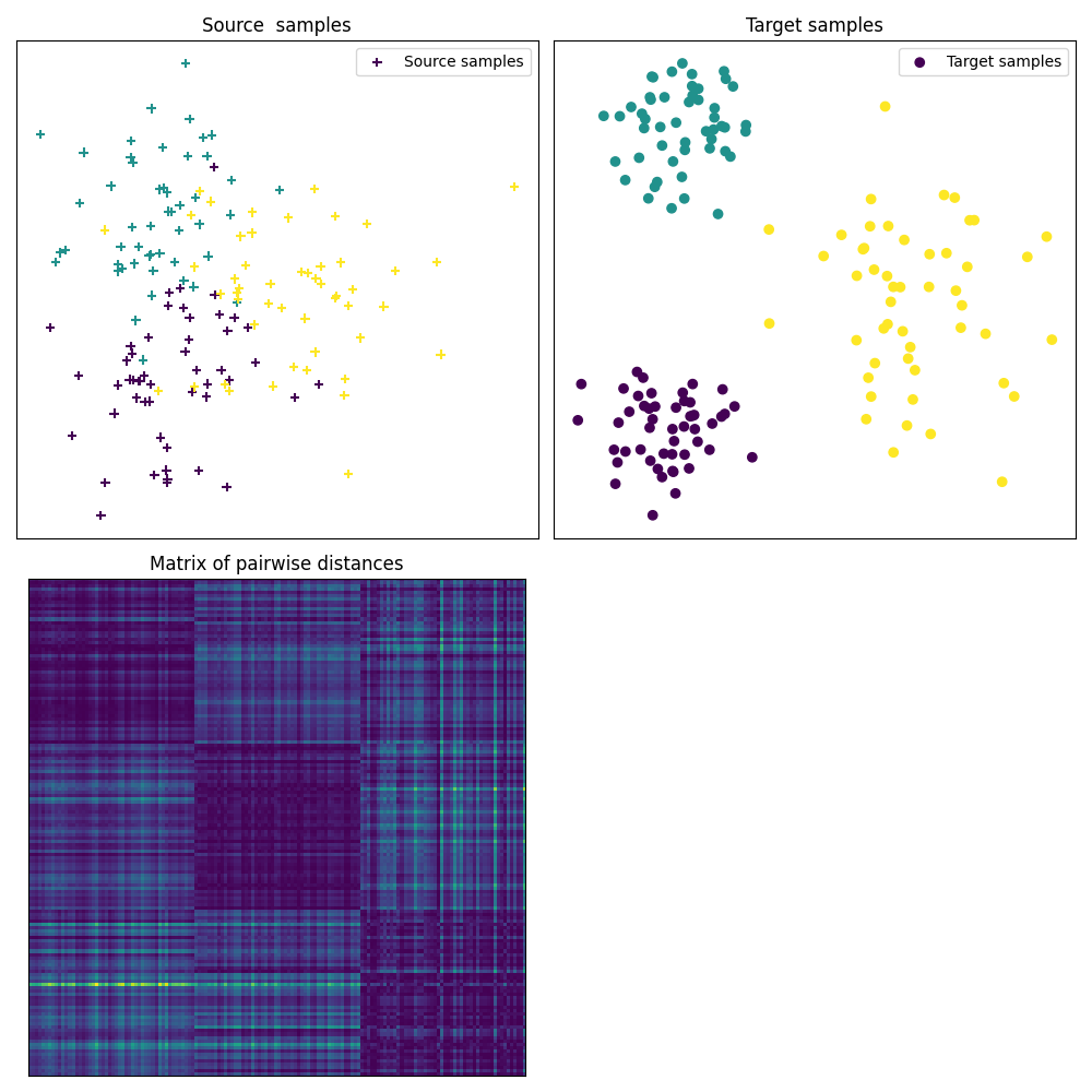
Fig 2 : plots optimal couplings for the different methods

pl.figure(2, figsize=(10, 6))

pl.subplot(2, 3, 1)
pl.imshow(ot_emd.coupling_, interpolation='nearest')
pl.xticks([])
pl.yticks([])
pl.title('Optimal coupling\nEMDTransport')

pl.subplot(2, 3, 2)
pl.imshow(ot_sinkhorn.coupling_, interpolation='nearest')
pl.xticks([])
pl.yticks([])
pl.title('Optimal coupling\nSinkhornTransport')

pl.subplot(2, 3, 3)
pl.imshow(ot_lpl1.coupling_, interpolation='nearest')
pl.xticks([])
pl.yticks([])
pl.title('Optimal coupling\nSinkhornLpl1Transport')

pl.subplot(2, 3, 4)
ot.plot.plot2D_samples_mat(Xs, Xt, ot_emd.coupling_, c=[.5, .5, 1])
pl.scatter(Xs[:, 0], Xs[:, 1], c=ys, marker='+', label='Source samples')
pl.scatter(Xt[:, 0], Xt[:, 1], c=yt, marker='o', label='Target samples')
pl.xticks([])
pl.yticks([])
pl.title('Main coupling coefficients\nEMDTransport')

pl.subplot(2, 3, 5)
ot.plot.plot2D_samples_mat(Xs, Xt, ot_sinkhorn.coupling_, c=[.5, .5, 1])
pl.scatter(Xs[:, 0], Xs[:, 1], c=ys, marker='+', label='Source samples')
pl.scatter(Xt[:, 0], Xt[:, 1], c=yt, marker='o', label='Target samples')
pl.xticks([])
pl.yticks([])
pl.title('Main coupling coefficients\nSinkhornTransport')

pl.subplot(2, 3, 6)
ot.plot.plot2D_samples_mat(Xs, Xt, ot_lpl1.coupling_, c=[.5, .5, 1])
pl.scatter(Xs[:, 0], Xs[:, 1], c=ys, marker='+', label='Source samples')
pl.scatter(Xt[:, 0], Xt[:, 1], c=yt, marker='o', label='Target samples')
pl.xticks([])
pl.yticks([])
pl.title('Main coupling coefficients\nSinkhornLpl1Transport')
pl.tight_layout()

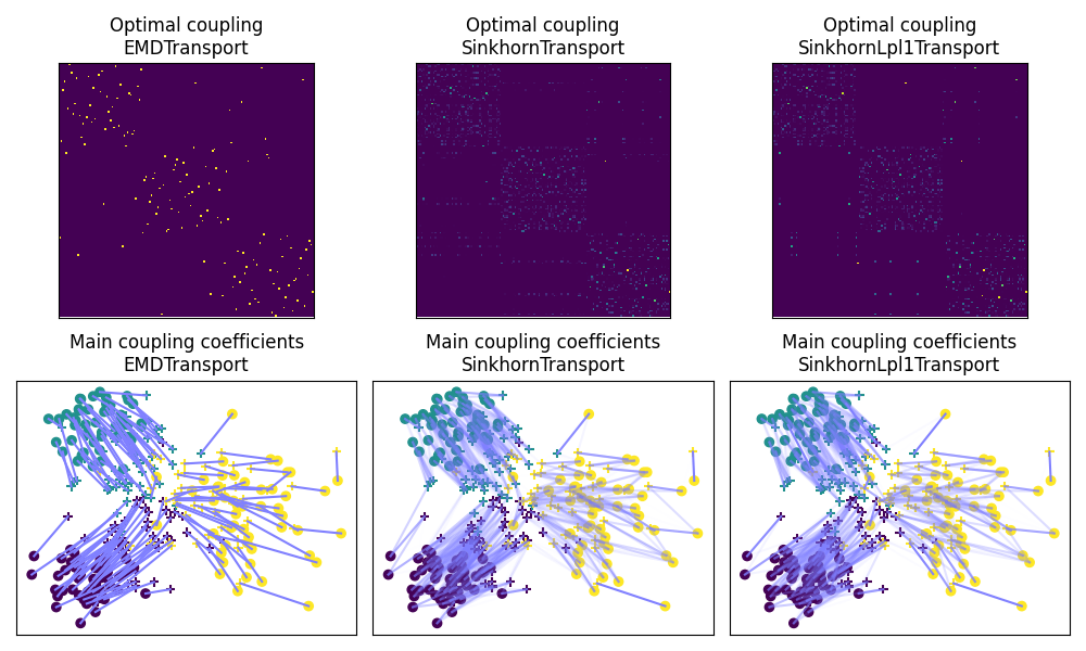
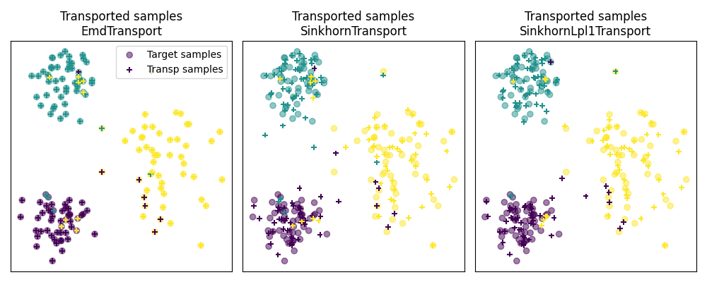
Fig 3 : plot transported samples

# display transported samples
pl.figure(4, figsize=(10, 4))
pl.subplot(1, 3, 1)
pl.scatter(Xt[:, 0], Xt[:, 1], c=yt, marker='o',
           label='Target samples', alpha=0.5)
pl.scatter(transp_Xs_emd[:, 0], transp_Xs_emd[:, 1], c=ys,
           marker='+', label='Transp samples', s=30)
pl.title('Transported samples\nEmdTransport')
pl.legend(loc=0)
pl.xticks([])
pl.yticks([])

pl.subplot(1, 3, 2)
pl.scatter(Xt[:, 0], Xt[:, 1], c=yt, marker='o',
           label='Target samples', alpha=0.5)
pl.scatter(transp_Xs_sinkhorn[:, 0], transp_Xs_sinkhorn[:, 1], c=ys,
           marker='+', label='Transp samples', s=30)
pl.title('Transported samples\nSinkhornTransport')
pl.xticks([])
pl.yticks([])

pl.subplot(1, 3, 3)
pl.scatter(Xt[:, 0], Xt[:, 1], c=yt, marker='o',
           label='Target samples', alpha=0.5)
pl.scatter(transp_Xs_lpl1[:, 0], transp_Xs_lpl1[:, 1], c=ys,
           marker='+', label='Transp samples', s=30)
pl.title('Transported samples\nSinkhornLpl1Transport')
pl.xticks([])
pl.yticks([])

pl.tight_layout()
pl.show()