Linear OT mapping estimation

# Author: Remi Flamary <remi.flamary@unice.fr>
#
# License: MIT License

# sphinx_gallery_thumbnail_number = 2

import os
from pathlib import Path

import numpy as np
from matplotlib import pyplot as plt
import ot

Generate data

n = 1000
d = 2
sigma = .1

rng = np.random.RandomState(42)

# source samples
angles = rng.rand(n, 1) * 2 * np.pi
xs = np.concatenate((np.sin(angles), np.cos(angles)),
                    axis=1) + sigma * rng.randn(n, 2)
xs[:n // 2, 1] += 2


# target samples
anglet = rng.rand(n, 1) * 2 * np.pi
xt = np.concatenate((np.sin(anglet), np.cos(anglet)),
                    axis=1) + sigma * rng.randn(n, 2)
xt[:n // 2, 1] += 2


A = np.array([[1.5, .7], [.7, 1.5]])
b = np.array([[4, 2]])
xt = xt.dot(A) + b

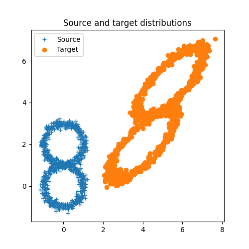
Plot data

plt.figure(1, (5, 5))
plt.plot(xs[:, 0], xs[:, 1], '+')
plt.plot(xt[:, 0], xt[:, 1], 'o')
plt.legend(('Source', 'Target'))
plt.title('Source and target distributions')
plt.show()

Estimate linear mapping and transport

# Gaussian (linear) Monge mapping estimation
Ae, be = ot.gaussian.empirical_bures_wasserstein_mapping(xs, xt)

xst = xs.dot(Ae) + be

# Gaussian (linear) GW mapping estimation
Agw, bgw = ot.gaussian.empirical_gaussian_gromov_wasserstein_mapping(xs, xt)

xstgw = xs.dot(Agw) + bgw

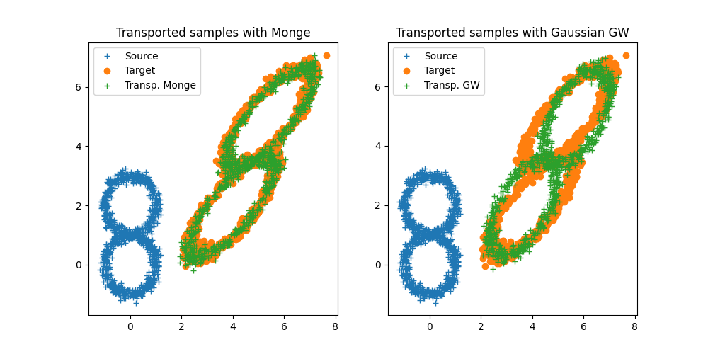
Plot transported samples

plt.figure(2, (10, 5))
plt.clf()
plt.subplot(1, 2, 1)
plt.plot(xs[:, 0], xs[:, 1], '+')
plt.plot(xt[:, 0], xt[:, 1], 'o')
plt.plot(xst[:, 0], xst[:, 1], '+')
plt.legend(('Source', 'Target', 'Transp. Monge'), loc=0)
plt.title('Transported samples with Monge')
plt.subplot(1, 2, 2)
plt.plot(xs[:, 0], xs[:, 1], '+')
plt.plot(xt[:, 0], xt[:, 1], 'o')
plt.plot(xstgw[:, 0], xstgw[:, 1], '+')
plt.legend(('Source', 'Target', 'Transp. GW'), loc=0)
plt.title('Transported samples with Gaussian GW')
plt.show()

Load image data

def im2mat(img):
    """Converts and image to matrix (one pixel per line)"""
    return img.reshape((img.shape[0] * img.shape[1], img.shape[2]))


def mat2im(X, shape):
    """Converts back a matrix to an image"""
    return X.reshape(shape)


def minmax(img):
    return np.clip(img, 0, 1)


# Loading images
this_file = os.path.realpath('__file__')
data_path = os.path.join(Path(this_file).parent.parent.parent, 'data')

I1 = plt.imread(os.path.join(data_path, 'ocean_day.jpg')).astype(np.float64) / 256
I2 = plt.imread(os.path.join(data_path, 'ocean_sunset.jpg')).astype(np.float64) / 256


X1 = im2mat(I1)
X2 = im2mat(I2)

Estimate mapping and adapt

# Monge mapping
mapping = ot.da.LinearTransport()
mapping.fit(Xs=X1, Xt=X2)


xst = mapping.transform(Xs=X1)
xts = mapping.inverse_transform(Xt=X2)

I1t = minmax(mat2im(xst, I1.shape))
I2t = minmax(mat2im(xts, I2.shape))

# gaussian GW mapping

mapping = ot.da.LinearGWTransport()
mapping.fit(Xs=X1, Xt=X2)


xstgw = mapping.transform(Xs=X1)
xtsgw = mapping.inverse_transform(Xt=X2)

I1tgw = minmax(mat2im(xstgw, I1.shape))
I2tgw = minmax(mat2im(xtsgw, I2.shape))

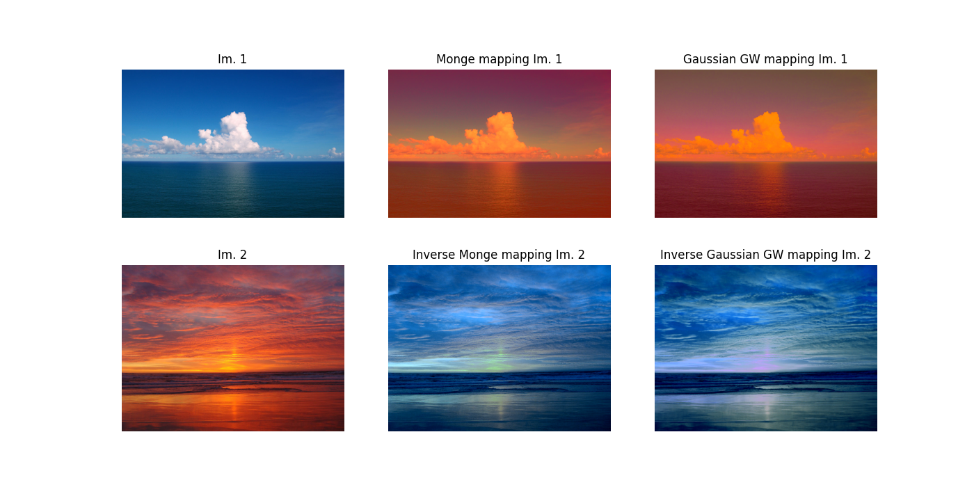
Plot transformed images

plt.figure(3, figsize=(14, 7))

plt.subplot(2, 3, 1)
plt.imshow(I1)
plt.axis('off')
plt.title('Im. 1')

plt.subplot(2, 3, 4)
plt.imshow(I2)
plt.axis('off')
plt.title('Im. 2')

plt.subplot(2, 3, 2)
plt.imshow(I1t)
plt.axis('off')
plt.title('Monge mapping Im. 1')

plt.subplot(2, 3, 5)
plt.imshow(I2t)
plt.axis('off')
plt.title('Inverse Monge mapping Im. 2')

plt.subplot(2, 3, 3)
plt.imshow(I1tgw)
plt.axis('off')
plt.title('Gaussian GW mapping Im. 1')

plt.subplot(2, 3, 6)
plt.imshow(I2tgw)
plt.axis('off')
plt.title('Inverse Gaussian GW mapping Im. 2')

Text(0.5, 1.0, 'Inverse Gaussian GW mapping Im. 2')