Note
Go to the end to download the full example code.
1D Wasserstein barycenter: exact LP vs entropic regularization
This example illustrates the computation of regularized Wasserstein Barycenter as proposed in [3] and exact LP barycenters using standard LP solver.
It reproduces approximately Figure 3.1 and 3.2 from the following paper: Cuturi, M., & Peyré, G. (2016). A smoothed dual approach for variational Wasserstein problems. SIAM Journal on Imaging Sciences, 9(1), 320-343.
[3] Benamou, J. D., Carlier, G., Cuturi, M., Nenna, L., & Peyré, G. (2015). Iterative Bregman projections for regularized transportation problems SIAM Journal on Scientific Computing, 37(2), A1111-A1138.
# Author: Remi Flamary <remi.flamary@unice.fr>
#
# License: MIT License

# sphinx_gallery_thumbnail_number = 4

import numpy as np
import matplotlib.pylab as pl
import ot

# necessary for 3d plot even if not used
from mpl_toolkits.mplot3d import Axes3D  # noqa
from matplotlib.collections import PolyCollection  # noqa

# import ot.lp.cvx as cvx
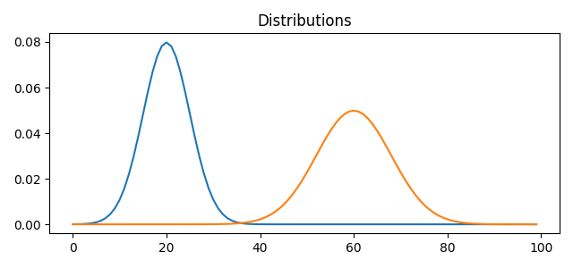
Gaussian Data
problems = []

n = 100  # nb bins

# bin positions
x = np.arange(n, dtype=np.float64)

# Gaussian distributions
# Gaussian distributions
a1 = ot.datasets.make_1D_gauss(n, m=20, s=5)  # m= mean, s= std
a2 = ot.datasets.make_1D_gauss(n, m=60, s=8)

# creating matrix A containing all distributions
A = np.vstack((a1, a2)).T
n_distributions = A.shape[1]

# loss matrix + normalization
M = ot.utils.dist0(n)
M /= M.max()
pl.figure(1, figsize=(6.4, 3))
for i in range(n_distributions):
    pl.plot(x, A[:, i])
pl.title("Distributions")
pl.tight_layout()
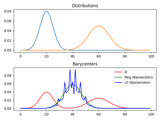
alpha = 0.5  # 0<=alpha<=1
weights = np.array([1 - alpha, alpha])

# l2bary
bary_l2 = A.dot(weights)

# wasserstein
reg = 1e-3
ot.tic()
bary_wass = ot.bregman.barycenter(A, M, reg, weights)
ot.toc()


ot.tic()
bary_wass2 = ot.lp.barycenter(A, M, weights)
ot.toc()

pl.figure(2)
pl.clf()
pl.subplot(2, 1, 1)
for i in range(n_distributions):
    pl.plot(x, A[:, i])
pl.title("Distributions")

pl.subplot(2, 1, 2)
pl.plot(x, bary_l2, "r", label="l2")
pl.plot(x, bary_wass, "g", label="Reg Wasserstein")
pl.plot(x, bary_wass2, "b", label="LP Wasserstein")
pl.legend()
pl.title("Barycenters")
pl.tight_layout()

problems.append([A, [bary_l2, bary_wass, bary_wass2]])
Elapsed time : 0.0035515429999577464 s
Elapsed time : 0.21948549499984438 s
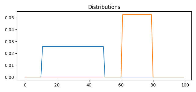
Stair Data
pl.figure(1, figsize=(6.4, 3))
for i in range(n_distributions):
    pl.plot(x, A[:, i])
pl.title("Distributions")
pl.tight_layout()
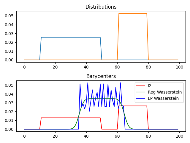
alpha = 0.5  # 0<=alpha<=1
weights = np.array([1 - alpha, alpha])

# l2bary
bary_l2 = A.dot(weights)

# wasserstein
reg = 1e-3
ot.tic()
bary_wass = ot.bregman.barycenter(A, M, reg, weights)
ot.toc()


ot.tic()
bary_wass2 = ot.lp.barycenter(A, M, weights)
ot.toc()


problems.append([A, [bary_l2, bary_wass, bary_wass2]])

pl.figure(2)
pl.clf()
pl.subplot(2, 1, 1)
for i in range(n_distributions):
    pl.plot(x, A[:, i])
pl.title("Distributions")

pl.subplot(2, 1, 2)
pl.plot(x, bary_l2, "r", label="l2")
pl.plot(x, bary_wass, "g", label="Reg Wasserstein")
pl.plot(x, bary_wass2, "b", label="LP Wasserstein")
pl.legend()
pl.title("Barycenters")
pl.tight_layout()
Elapsed time : 0.007610617999944225 s
Elapsed time : 0.1240881079997962 s
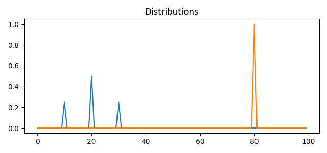
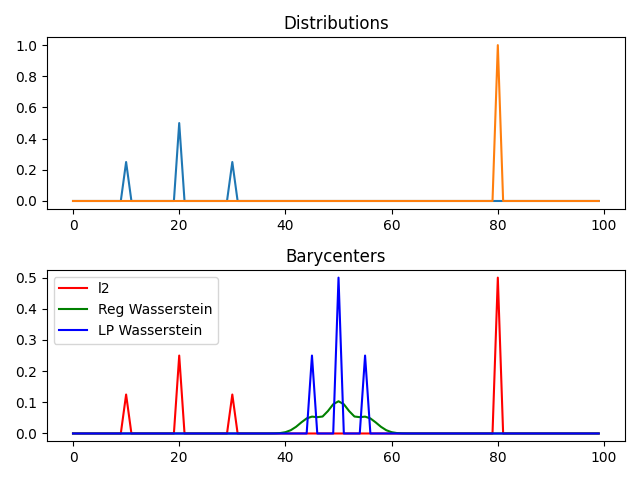
Dirac Data
pl.figure(1, figsize=(6.4, 3))
for i in range(n_distributions):
    pl.plot(x, A[:, i])
pl.title("Distributions")
pl.tight_layout()
alpha = 0.5  # 0<=alpha<=1
weights = np.array([1 - alpha, alpha])

# l2bary
bary_l2 = A.dot(weights)

# wasserstein
reg = 1e-3
ot.tic()
bary_wass = ot.bregman.barycenter(A, M, reg, weights)
ot.toc()


ot.tic()
bary_wass2 = ot.lp.barycenter(A, M, weights)
ot.toc()


problems.append([A, [bary_l2, bary_wass, bary_wass2]])

pl.figure(2)
pl.clf()
pl.subplot(2, 1, 1)
for i in range(n_distributions):
    pl.plot(x, A[:, i])
pl.title("Distributions")

pl.subplot(2, 1, 2)
pl.plot(x, bary_l2, "r", label="l2")
pl.plot(x, bary_wass, "g", label="Reg Wasserstein")
pl.plot(x, bary_wass2, "b", label="LP Wasserstein")
pl.legend()
pl.title("Barycenters")
pl.tight_layout()
Elapsed time : 0.001068939999640861 s
Elapsed time : 0.06673658800036719 s
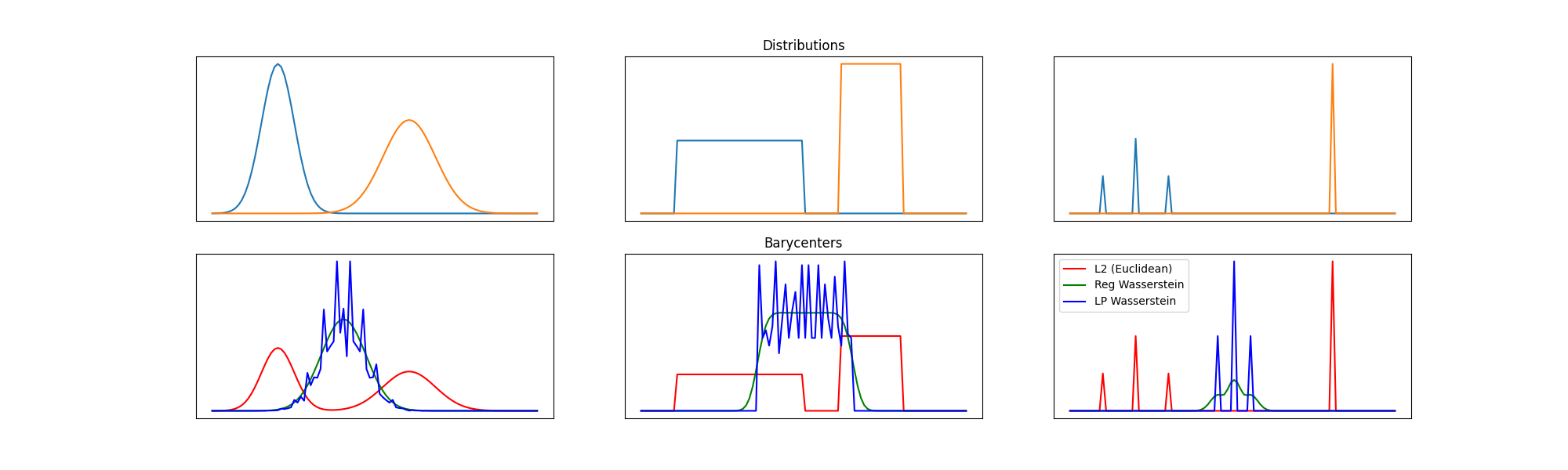
Final figure
nbm = len(problems)
nbm2 = nbm // 2


pl.figure(2, (20, 6))
pl.clf()

for i in range(nbm):
    A = problems[i][0]
    bary_l2 = problems[i][1][0]
    bary_wass = problems[i][1][1]
    bary_wass2 = problems[i][1][2]

    pl.subplot(2, nbm, 1 + i)
    for j in range(n_distributions):
        pl.plot(x, A[:, j])
    if i == nbm2:
        pl.title("Distributions")
    pl.xticks(())
    pl.yticks(())

    pl.subplot(2, nbm, 1 + i + nbm)

    pl.plot(x, bary_l2, "r", label="L2 (Euclidean)")
    pl.plot(x, bary_wass, "g", label="Reg Wasserstein")
    pl.plot(x, bary_wass2, "b", label="LP Wasserstein")
    if i == nbm - 1:
        pl.legend()
    if i == nbm2:
        pl.title("Barycenters")

    pl.xticks(())
    pl.yticks(())
Total running time of the script: (0 minutes 1.724 seconds)