ot.dr
Dimension reduction with OT
Warning
Note that by default the module is not imported in ot. In order to
use it you need to explicitly import ot.dr
Functions
- ot.dr.ewca(X, U0=None, reg=1, k=2, method='BCD', sinkhorn_method='sinkhorn', stopThr=1e-06, maxiter=100, maxiter_sink=1000, maxiter_MM=10, verbose=0)[source]
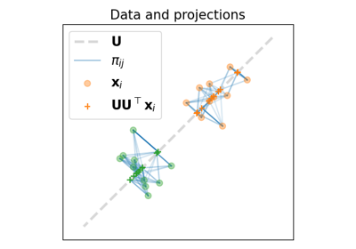
Entropic Wasserstein Component Analysis [52].
The function solves the following optimization problem:
\[\mathbf{U} = \mathop{\arg \min}_\mathbf{U} \quad W(\mathbf{X}, \mathbf{U}\mathbf{U}^T \mathbf{X})\]where :
\(\mathbf{U}\) is a matrix in the Stiefel(p, d) manifold
\(W\) is entropic regularized Wasserstein distances
\(\mathbf{X}\) are samples
- Parameters:
X (ndarray, shape (n, d)) – Samples from measure \(\mu\).
U0 (ndarray, shape (d, k), optional) – Initial starting point for projection.
reg (float, optional) – Regularization term >0 (entropic regularization).
k (int, optional) – Subspace dimension.
method (str, optional) – Eather ‘BCD’ or ‘MM’ (Block Coordinate Descent or Majorization-Minimization). Prefer MM when d is large.
sinkhorn_method (str) – Method used for the Sinkhorn solver, see ot.bregman.sinkhorn for more details.
stopThr (float, optional) – Stop threshold on error (>0).
maxiter (int, optional) – Maximum number of iterations of the BCD/MM.
maxiter_sink (int, optional) – Maximum number of iterations of the Sinkhorn solver.
maxiter_MM (int, optional) – Maximum number of iterations of the MM (only used when method=’MM’).
verbose (int, optional) – Print information along iterations.
- Returns:
pi (ndarray, shape (n, n)) – Optimal transportation matrix for the given parameters.
U (ndarray, shape (d, k)) – Matrix Stiefel manifold.
References
Examples using ot.dr.ewca
Examples using ot.dr.fda
- ot.dr.logsumexp(M, axis)[source]
Log-sum-exp reduction compatible with autograd (no numpy implementation)
- ot.dr.projection_robust_wasserstein(X, Y, a, b, tau, U0=None, reg=0.1, k=2, stopThr=0.001, maxiter=100, verbose=0, random_state=None)[source]
Projection Robust Wasserstein Distance [32]
The function solves the following optimization problem:
\[\max_{U \in St(d, k)} \ \min_{\pi \in \Pi(\mu,\nu)} \quad \sum_{i,j} \pi_{i,j} \|U^T(\mathbf{x}_i - \mathbf{y}_j)\|^2 - \mathrm{reg} \cdot H(\pi)\]\(U\) is a linear projection operator in the Stiefel(d, k) manifold
\(H(\pi)\) is entropy regularizer
\(\mathbf{x}_i\), \(\mathbf{y}_j\) are samples of measures \(\mu\) and \(\nu\) respectively
- Parameters:
X (ndarray, shape (n, d)) – Samples from measure \(\mu\)
Y (ndarray, shape (n, d)) – Samples from measure \(\nu\)
a (ndarray, shape (n, )) – weights for measure \(\mu\)
b (ndarray, shape (n, )) – weights for measure \(\nu\)
tau (float) – stepsize for Riemannian Gradient Descent
U0 (ndarray, shape (d, p)) – Initial starting point for projection.
reg (float, optional) – Regularization term >0 (entropic regularization)
k (int) – Subspace dimension
stopThr (float, optional) – Stop threshold on error (>0)
verbose (int, optional) – Print information along iterations.
random_state (int, RandomState instance or None, default=None) – Determines random number generation for initial value of projection operator when U0 is not given.
- Returns:
pi (ndarray, shape (n, n)) – Optimal transportation matrix for the given parameters
U (ndarray, shape (d, k)) – Projection operator.
References
- ot.dr.sinkhorn(w1, w2, M, reg, k)[source]
Sinkhorn algorithm with fixed number of iteration (autograd)
- ot.dr.sinkhorn_log(w1, w2, M, reg, k)[source]
Sinkhorn algorithm in log-domain with fixed number of iteration (autograd)
- ot.dr.wda(X, y, p=2, reg=1, k=10, solver=None, sinkhorn_method='sinkhorn', maxiter=100, verbose=0, P0=None, normalize=False)[source]
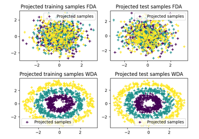
Wasserstein Discriminant Analysis [11]
The function solves the following optimization problem:
\[\mathbf{P} = \mathop{\arg \min}_\mathbf{P} \quad \frac{\sum\limits_i W(P \mathbf{X}^i, P \mathbf{X}^i)}{\sum\limits_{i, j \neq i} W(P \mathbf{X}^i, P \mathbf{X}^j)}\]where :
\(P\) is a linear projection operator in the Stiefel(p, d) manifold
\(W\) is entropic regularized Wasserstein distances
\(\mathbf{X}^i\) are samples in the dataset corresponding to class i
Choosing a Sinkhorn solver
By default and when using a regularization parameter that is not too small the default sinkhorn solver should be enough. If you need to use a small regularization to get sparse cost matrices, you should use the
ot.dr.sinkhorn_log()solver that will avoid numerical errors, but can be slow in practice.- Parameters:
X (ndarray, shape (n, d)) – Training samples.
y (ndarray, shape (n,)) – Labels for training samples.
p (int, optional) – Size of dimensionality reduction.
reg (float, optional) – Regularization term >0 (entropic regularization)
solver (None | str, optional) – None for steepest descent or ‘TrustRegions’ for trust regions algorithm else should be a pymanopt.solvers
sinkhorn_method (str) – method used for the Sinkhorn solver, either ‘sinkhorn’ or ‘sinkhorn_log’
P0 (ndarray, shape (d, p)) – Initial starting point for projection.
normalize (bool, optional) – Normalize the Wasserstaiun distance by the average distance on P0 (default : False)
verbose (int, optional) – Print information along iterations.
- Returns:
P (ndarray, shape (d, p)) – Optimal transportation matrix for the given parameters
proj (callable) – Projection function including mean centering.
References
Examples using ot.dr.wda
- ot.dr.ewca(X, U0=None, reg=1, k=2, method='BCD', sinkhorn_method='sinkhorn', stopThr=1e-06, maxiter=100, maxiter_sink=1000, maxiter_MM=10, verbose=0)[source]
Entropic Wasserstein Component Analysis [52].
The function solves the following optimization problem:
\[\mathbf{U} = \mathop{\arg \min}_\mathbf{U} \quad W(\mathbf{X}, \mathbf{U}\mathbf{U}^T \mathbf{X})\]where :
\(\mathbf{U}\) is a matrix in the Stiefel(p, d) manifold
\(W\) is entropic regularized Wasserstein distances
\(\mathbf{X}\) are samples
- Parameters:
X (ndarray, shape (n, d)) – Samples from measure \(\mu\).
U0 (ndarray, shape (d, k), optional) – Initial starting point for projection.
reg (float, optional) – Regularization term >0 (entropic regularization).
k (int, optional) – Subspace dimension.
method (str, optional) – Eather ‘BCD’ or ‘MM’ (Block Coordinate Descent or Majorization-Minimization). Prefer MM when d is large.
sinkhorn_method (str) – Method used for the Sinkhorn solver, see ot.bregman.sinkhorn for more details.
stopThr (float, optional) – Stop threshold on error (>0).
maxiter (int, optional) – Maximum number of iterations of the BCD/MM.
maxiter_sink (int, optional) – Maximum number of iterations of the Sinkhorn solver.
maxiter_MM (int, optional) – Maximum number of iterations of the MM (only used when method=’MM’).
verbose (int, optional) – Print information along iterations.
- Returns:
pi (ndarray, shape (n, n)) – Optimal transportation matrix for the given parameters.
U (ndarray, shape (d, k)) – Matrix Stiefel manifold.
References
- ot.dr.fda(X, y, p=2, reg=1e-16)[source]
Fisher Discriminant Analysis
- Parameters:
- Returns:
P (ndarray, shape (d, p)) – Optimal transportation matrix for the given parameters
proj (callable) – projection function including mean centering
- ot.dr.logsumexp(M, axis)[source]
Log-sum-exp reduction compatible with autograd (no numpy implementation)
- ot.dr.projection_robust_wasserstein(X, Y, a, b, tau, U0=None, reg=0.1, k=2, stopThr=0.001, maxiter=100, verbose=0, random_state=None)[source]
Projection Robust Wasserstein Distance [32]
The function solves the following optimization problem:
\[\max_{U \in St(d, k)} \ \min_{\pi \in \Pi(\mu,\nu)} \quad \sum_{i,j} \pi_{i,j} \|U^T(\mathbf{x}_i - \mathbf{y}_j)\|^2 - \mathrm{reg} \cdot H(\pi)\]\(U\) is a linear projection operator in the Stiefel(d, k) manifold
\(H(\pi)\) is entropy regularizer
\(\mathbf{x}_i\), \(\mathbf{y}_j\) are samples of measures \(\mu\) and \(\nu\) respectively
- Parameters:
X (ndarray, shape (n, d)) – Samples from measure \(\mu\)
Y (ndarray, shape (n, d)) – Samples from measure \(\nu\)
a (ndarray, shape (n, )) – weights for measure \(\mu\)
b (ndarray, shape (n, )) – weights for measure \(\nu\)
tau (float) – stepsize for Riemannian Gradient Descent
U0 (ndarray, shape (d, p)) – Initial starting point for projection.
reg (float, optional) – Regularization term >0 (entropic regularization)
k (int) – Subspace dimension
stopThr (float, optional) – Stop threshold on error (>0)
verbose (int, optional) – Print information along iterations.
random_state (int, RandomState instance or None, default=None) – Determines random number generation for initial value of projection operator when U0 is not given.
- Returns:
pi (ndarray, shape (n, n)) – Optimal transportation matrix for the given parameters
U (ndarray, shape (d, k)) – Projection operator.
References
- ot.dr.sinkhorn(w1, w2, M, reg, k)[source]
Sinkhorn algorithm with fixed number of iteration (autograd)
- ot.dr.sinkhorn_log(w1, w2, M, reg, k)[source]
Sinkhorn algorithm in log-domain with fixed number of iteration (autograd)
- ot.dr.wda(X, y, p=2, reg=1, k=10, solver=None, sinkhorn_method='sinkhorn', maxiter=100, verbose=0, P0=None, normalize=False)[source]
Wasserstein Discriminant Analysis [11]
The function solves the following optimization problem:
\[\mathbf{P} = \mathop{\arg \min}_\mathbf{P} \quad \frac{\sum\limits_i W(P \mathbf{X}^i, P \mathbf{X}^i)}{\sum\limits_{i, j \neq i} W(P \mathbf{X}^i, P \mathbf{X}^j)}\]where :
\(P\) is a linear projection operator in the Stiefel(p, d) manifold
\(W\) is entropic regularized Wasserstein distances
\(\mathbf{X}^i\) are samples in the dataset corresponding to class i
Choosing a Sinkhorn solver
By default and when using a regularization parameter that is not too small the default sinkhorn solver should be enough. If you need to use a small regularization to get sparse cost matrices, you should use the
ot.dr.sinkhorn_log()solver that will avoid numerical errors, but can be slow in practice.- Parameters:
X (ndarray, shape (n, d)) – Training samples.
y (ndarray, shape (n,)) – Labels for training samples.
p (int, optional) – Size of dimensionality reduction.
reg (float, optional) – Regularization term >0 (entropic regularization)
solver (None | str, optional) – None for steepest descent or ‘TrustRegions’ for trust regions algorithm else should be a pymanopt.solvers
sinkhorn_method (str) – method used for the Sinkhorn solver, either ‘sinkhorn’ or ‘sinkhorn_log’
P0 (ndarray, shape (d, p)) – Initial starting point for projection.
normalize (bool, optional) – Normalize the Wasserstaiun distance by the average distance on P0 (default : False)
verbose (int, optional) – Print information along iterations.
- Returns:
P (ndarray, shape (d, p)) – Optimal transportation matrix for the given parameters
proj (callable) – Projection function including mean centering.
References