Partial Wasserstein and Gromov-Wasserstein example

This example is designed to show how to use the Partial (Gromov-)Wasserstein distance computation in POT.

# Author: Laetitia Chapel <laetitia.chapel@irisa.fr>
# License: MIT License

# sphinx_gallery_thumbnail_number = 2

# necessary for 3d plot even if not used
from mpl_toolkits.mplot3d import Axes3D  # noqa
import scipy as sp
import numpy as np
import matplotlib.pylab as pl
import ot

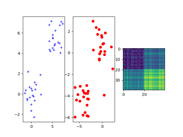
Sample two 2D Gaussian distributions and plot them

For demonstration purpose, we sample two Gaussian distributions in 2-d spaces and add some random noise.

n_samples = 20  # nb samples (gaussian)
n_noise = 20  # nb of samples (noise)

mu = np.array([0, 0])
cov = np.array([[1, 0], [0, 2]])

xs = ot.datasets.make_2D_samples_gauss(n_samples, mu, cov)
xs = np.append(xs, (np.random.rand(n_noise, 2) + 1) * 4).reshape((-1, 2))
xt = ot.datasets.make_2D_samples_gauss(n_samples, mu, cov)
xt = np.append(xt, (np.random.rand(n_noise, 2) + 1) * -3).reshape((-1, 2))

M = sp.spatial.distance.cdist(xs, xt)

fig = pl.figure()
ax1 = fig.add_subplot(131)
ax1.plot(xs[:, 0], xs[:, 1], '+b', label='Source samples')
ax2 = fig.add_subplot(132)
ax2.scatter(xt[:, 0], xt[:, 1], color='r')
ax3 = fig.add_subplot(133)
ax3.imshow(M)
pl.show()

Compute partial Wasserstein plans and distance

p = ot.unif(n_samples + n_noise)
q = ot.unif(n_samples + n_noise)

w0, log0 = ot.partial.partial_wasserstein(p, q, M, m=0.5, log=True)
w, log = ot.partial.entropic_partial_wasserstein(p, q, M, reg=0.1, m=0.5,
                                                 log=True)

print('Partial Wasserstein distance (m = 0.5): ' + str(log0['partial_w_dist']))
print('Entropic partial Wasserstein distance (m = 0.5): ' +
      str(log['partial_w_dist']))

pl.figure(1, (10, 5))
pl.subplot(1, 2, 1)
pl.imshow(w0, cmap='jet')
pl.title('Partial Wasserstein')
pl.subplot(1, 2, 2)
pl.imshow(w, cmap='jet')
pl.title('Entropic partial Wasserstein')
pl.show()

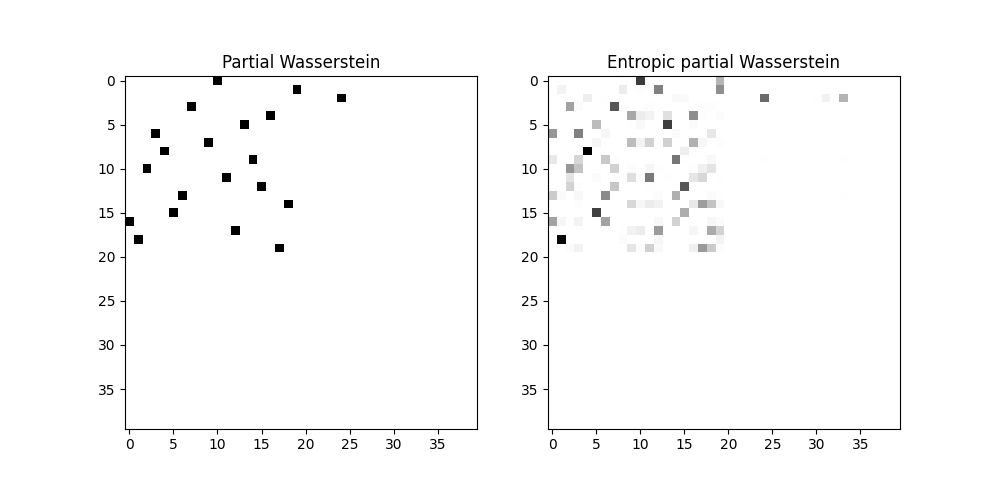
Partial Wasserstein distance (m = 0.5): 0.47910182636916243
Entropic partial Wasserstein distance (m = 0.5): 0.5034205945081646

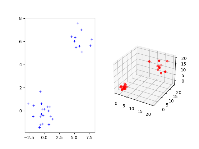
Sample one 2D and 3D Gaussian distributions and plot them

The Gromov-Wasserstein distance allows to compute distances with samples that do not belong to the same metric space. For demonstration purpose, we sample two Gaussian distributions in 2- and 3-dimensional spaces.

n_samples = 20  # nb samples
n_noise = 10  # nb of samples (noise)

p = ot.unif(n_samples + n_noise)
q = ot.unif(n_samples + n_noise)

mu_s = np.array([0, 0])
cov_s = np.array([[1, 0], [0, 1]])

mu_t = np.array([0, 0, 0])
cov_t = np.array([[1, 0, 0], [0, 1, 0], [0, 0, 1]])


xs = ot.datasets.make_2D_samples_gauss(n_samples, mu_s, cov_s)
xs = np.concatenate((xs, ((np.random.rand(n_noise, 2) + 1) * 4)), axis=0)
P = sp.linalg.sqrtm(cov_t)
xt = np.random.randn(n_samples, 3).dot(P) + mu_t
xt = np.concatenate((xt, ((np.random.rand(n_noise, 3) + 1) * 10)), axis=0)

fig = pl.figure()
ax1 = fig.add_subplot(121)
ax1.plot(xs[:, 0], xs[:, 1], '+b', label='Source samples')
ax2 = fig.add_subplot(122, projection='3d')
ax2.scatter(xt[:, 0], xt[:, 1], xt[:, 2], color='r')
pl.show()

Compute partial Gromov-Wasserstein plans and distance

C1 = sp.spatial.distance.cdist(xs, xs)
C2 = sp.spatial.distance.cdist(xt, xt)

# transport 100% of the mass
print('------m = 1')
m = 1
res0, log0 = ot.partial.partial_gromov_wasserstein(C1, C2, p, q, m=m, log=True)
res, log = ot.partial.entropic_partial_gromov_wasserstein(C1, C2, p, q, 10,
                                                          m=m, log=True,
                                                          verbose=True)

print('Wasserstein distance (m = 1): ' + str(log0['partial_gw_dist']))
print('Entropic Wasserstein distance (m = 1): ' + str(log['partial_gw_dist']))

pl.figure(1, (10, 5))
pl.title("mass to be transported m = 1")
pl.subplot(1, 2, 1)
pl.imshow(res0, cmap='jet')
pl.title('Gromov-Wasserstein')
pl.subplot(1, 2, 2)
pl.imshow(res, cmap='jet')
pl.title('Entropic Gromov-Wasserstein')
pl.show()

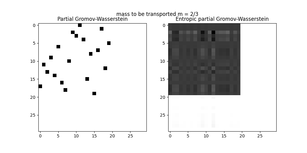
# transport 2/3 of the mass
print('------m = 2/3')
m = 2 / 3
res0, log0 = ot.partial.partial_gromov_wasserstein(C1, C2, p, q, m=m, log=True,
                                                   verbose=True)
res, log = ot.partial.entropic_partial_gromov_wasserstein(C1, C2, p, q, 10,
                                                          m=m, log=True,
                                                          verbose=True)

print('Partial Wasserstein distance (m = 2/3): ' +
      str(log0['partial_gw_dist']))
print('Entropic partial Wasserstein distance (m = 2/3): ' +
      str(log['partial_gw_dist']))

pl.figure(1, (10, 5))
pl.title("mass to be transported m = 2/3")
pl.subplot(1, 2, 1)
pl.imshow(res0, cmap='jet')
pl.title('Partial Gromov-Wasserstein')
pl.subplot(1, 2, 2)
pl.imshow(res, cmap='jet')
pl.title('Entropic partial Gromov-Wasserstein')
pl.show()

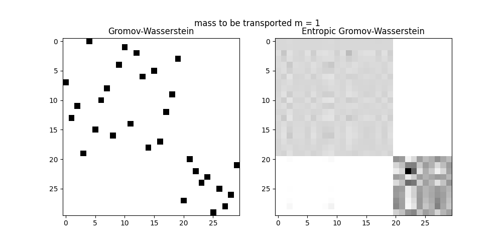
------m = 1
It.  |Err         |Loss
-------------------------------
    0|2.611280e-02|8.345385e+01
   10|8.584346e-15|6.659015e+01
Wasserstein distance (m = 1): 65.38071035222889
Entropic Wasserstein distance (m = 1): 66.59015303098326
------m = 2/3
It.  |Err         |Loss
-------------------------------
    0|1.478237e-01|5.894947e+00
It.  |Err         |Loss
-------------------------------
    0|2.251769e-02|6.596705e+00
   10|1.808371e-07|9.136110e-01
   20|1.859072e-14|9.136043e-01
Partial Wasserstein distance (m = 2/3): 0.11743971783944865
Entropic partial Wasserstein distance (m = 2/3): 0.9136043100219415