OT for image color adaptation

This example presents a way of transferring colors between two images with Optimal Transport as introduced in [6]

[6] Ferradans, S., Papadakis, N., Peyre, G., & Aujol, J. F. (2014). Regularized discrete optimal transport. SIAM Journal on Imaging Sciences, 7(3), 1853-1882.

# Authors: Remi Flamary <remi.flamary@unice.fr>
#          Stanislas Chambon <stan.chambon@gmail.com>
#
# License: MIT License

# sphinx_gallery_thumbnail_number = 2

import os
from pathlib import Path

import numpy as np
from matplotlib import pyplot as plt
import ot


rng = np.random.RandomState(42)


def im2mat(img):
    """Converts an image to matrix (one pixel per line)"""
    return img.reshape((img.shape[0] * img.shape[1], img.shape[2]))


def mat2im(X, shape):
    """Converts back a matrix to an image"""
    return X.reshape(shape)


def minmax(img):
    return np.clip(img, 0, 1)

Generate data

# Loading images
this_file = os.path.realpath('__file__')
data_path = os.path.join(Path(this_file).parent.parent.parent, 'data')

I1 = plt.imread(os.path.join(data_path, 'ocean_day.jpg')).astype(np.float64) / 256
I2 = plt.imread(os.path.join(data_path, 'ocean_sunset.jpg')).astype(np.float64) / 256

X1 = im2mat(I1)
X2 = im2mat(I2)

# training samples
nb = 500
idx1 = rng.randint(X1.shape[0], size=(nb,))
idx2 = rng.randint(X2.shape[0], size=(nb,))

Xs = X1[idx1, :]
Xt = X2[idx2, :]

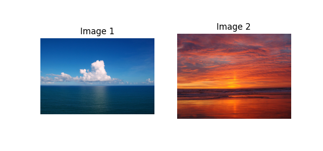
Plot original image

plt.figure(1, figsize=(6.4, 3))

plt.subplot(1, 2, 1)
plt.imshow(I1)
plt.axis('off')
plt.title('Image 1')

plt.subplot(1, 2, 2)
plt.imshow(I2)
plt.axis('off')
plt.title('Image 2')

Text(0.5, 1.0, 'Image 2')

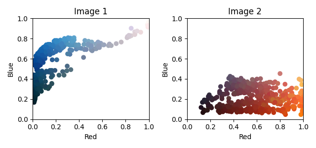
Scatter plot of colors

plt.figure(2, figsize=(6.4, 3))

plt.subplot(1, 2, 1)
plt.scatter(Xs[:, 0], Xs[:, 2], c=Xs)
plt.axis([0, 1, 0, 1])
plt.xlabel('Red')
plt.ylabel('Blue')
plt.title('Image 1')

plt.subplot(1, 2, 2)
plt.scatter(Xt[:, 0], Xt[:, 2], c=Xt)
plt.axis([0, 1, 0, 1])
plt.xlabel('Red')
plt.ylabel('Blue')
plt.title('Image 2')
plt.tight_layout()

Instantiate the different transport algorithms and fit them

# EMDTransport
ot_emd = ot.da.EMDTransport()
ot_emd.fit(Xs=Xs, Xt=Xt)

# SinkhornTransport
ot_sinkhorn = ot.da.SinkhornTransport(reg_e=1e-1)
ot_sinkhorn.fit(Xs=Xs, Xt=Xt)

# prediction between images (using out of sample prediction as in [6])
transp_Xs_emd = ot_emd.transform(Xs=X1)
transp_Xt_emd = ot_emd.inverse_transform(Xt=X2)

transp_Xs_sinkhorn = ot_sinkhorn.transform(Xs=X1)
transp_Xt_sinkhorn = ot_sinkhorn.inverse_transform(Xt=X2)

I1t = minmax(mat2im(transp_Xs_emd, I1.shape))
I2t = minmax(mat2im(transp_Xt_emd, I2.shape))

I1te = minmax(mat2im(transp_Xs_sinkhorn, I1.shape))
I2te = minmax(mat2im(transp_Xt_sinkhorn, I2.shape))

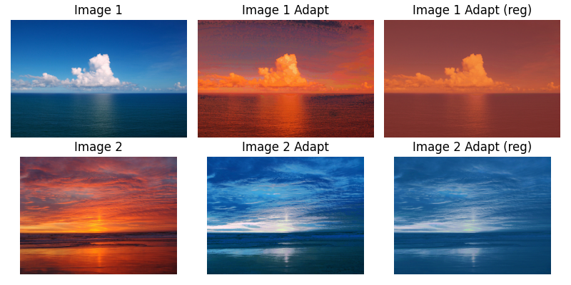
Plot new images

plt.figure(3, figsize=(8, 4))

plt.subplot(2, 3, 1)
plt.imshow(I1)
plt.axis('off')
plt.title('Image 1')

plt.subplot(2, 3, 2)
plt.imshow(I1t)
plt.axis('off')
plt.title('Image 1 Adapt')

plt.subplot(2, 3, 3)
plt.imshow(I1te)
plt.axis('off')
plt.title('Image 1 Adapt (reg)')

plt.subplot(2, 3, 4)
plt.imshow(I2)
plt.axis('off')
plt.title('Image 2')

plt.subplot(2, 3, 5)
plt.imshow(I2t)
plt.axis('off')
plt.title('Image 2 Adapt')

plt.subplot(2, 3, 6)
plt.imshow(I2te)
plt.axis('off')
plt.title('Image 2 Adapt (reg)')
plt.tight_layout()

plt.show()