OT for domain adaptation

This example introduces a domain adaptation in a 2D setting and the 4 OTDA approaches currently supported in POT.

# Authors: Remi Flamary <remi.flamary@unice.fr>
#          Stanislas Chambon <stan.chambon@gmail.com>
#
# License: MIT License

import matplotlib.pylab as pl
import ot

Generate data

n_source_samples = 150
n_target_samples = 150

Xs, ys = ot.datasets.make_data_classif('3gauss', n_source_samples)
Xt, yt = ot.datasets.make_data_classif('3gauss2', n_target_samples)

Instantiate the different transport algorithms and fit them

# EMD Transport
ot_emd = ot.da.EMDTransport()
ot_emd.fit(Xs=Xs, Xt=Xt)

# Sinkhorn Transport
ot_sinkhorn = ot.da.SinkhornTransport(reg_e=1e-1)
ot_sinkhorn.fit(Xs=Xs, Xt=Xt)

# Sinkhorn Transport with Group lasso regularization
ot_lpl1 = ot.da.SinkhornLpl1Transport(reg_e=1e-1, reg_cl=1e0)
ot_lpl1.fit(Xs=Xs, ys=ys, Xt=Xt)

# Sinkhorn Transport with Group lasso regularization l1l2
ot_l1l2 = ot.da.SinkhornL1l2Transport(reg_e=1e-1, reg_cl=2e0, max_iter=20,
                                      verbose=True)
ot_l1l2.fit(Xs=Xs, ys=ys, Xt=Xt)

# transport source samples onto target samples
transp_Xs_emd = ot_emd.transform(Xs=Xs)
transp_Xs_sinkhorn = ot_sinkhorn.transform(Xs=Xs)
transp_Xs_lpl1 = ot_lpl1.transform(Xs=Xs)
transp_Xs_l1l2 = ot_l1l2.transform(Xs=Xs)

/home/circleci/project/ot/bregman/_sinkhorn.py:531: UserWarning: Sinkhorn did not converge. You might want to increase the number of iterations `numItermax` or the regularization parameter `reg`.
  warnings.warn("Sinkhorn did not converge. You might want to "
It.  |Loss        |Relative loss|Absolute loss
------------------------------------------------
    0|9.763061e+00|0.000000e+00|0.000000e+00
    1|2.081861e+00|3.689583e+00|7.681200e+00
    2|1.862280e+00|1.179100e-01|2.195813e-01
    3|1.821987e+00|2.211501e-02|4.029326e-02
    4|1.808932e+00|7.216608e-03|1.305436e-02
    5|1.792762e+00|9.019666e-03|1.617012e-02
    6|1.785968e+00|3.804295e-03|6.794348e-03
    7|1.778259e+00|4.335304e-03|7.709292e-03
    8|1.772608e+00|3.187777e-03|5.650678e-03
    9|1.768734e+00|2.190456e-03|3.874332e-03
   10|1.768700e+00|1.876119e-05|3.318292e-05
   11|1.767482e+00|6.894485e-04|1.218588e-03
   12|1.765491e+00|1.127725e-03|1.990989e-03
   13|1.762434e+00|1.734384e-03|3.056738e-03
   14|1.759833e+00|1.478250e-03|2.601472e-03
   15|1.758374e+00|8.294698e-04|1.458518e-03
   16|1.757601e+00|4.396351e-04|7.727032e-04
   17|1.756624e+00|5.562652e-04|9.771489e-04
   18|1.754377e+00|1.281229e-03|2.247758e-03
   19|1.753747e+00|3.587988e-04|6.292424e-04
It.  |Loss        |Relative loss|Absolute loss
------------------------------------------------
   20|1.753162e+00|3.336538e-04|5.849492e-04

Fig 1 : plots source and target samples

pl.figure(1, figsize=(10, 5))
pl.subplot(1, 2, 1)
pl.scatter(Xs[:, 0], Xs[:, 1], c=ys, marker='+', label='Source samples')
pl.xticks([])
pl.yticks([])
pl.legend(loc=0)
pl.title('Source  samples')

pl.subplot(1, 2, 2)
pl.scatter(Xt[:, 0], Xt[:, 1], c=yt, marker='o', label='Target samples')
pl.xticks([])
pl.yticks([])
pl.legend(loc=0)
pl.title('Target samples')
pl.tight_layout()

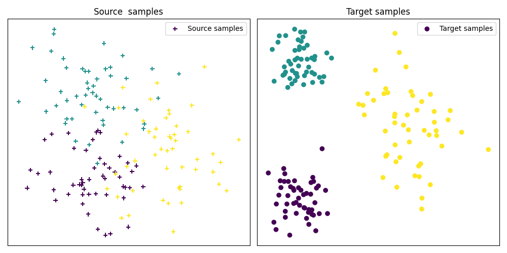
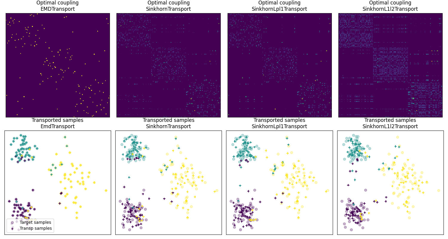
Fig 2 : plot optimal couplings and transported samples

param_img = {'interpolation': 'nearest'}

pl.figure(2, figsize=(15, 8))
pl.subplot(2, 4, 1)
pl.imshow(ot_emd.coupling_, **param_img)
pl.xticks([])
pl.yticks([])
pl.title('Optimal coupling\nEMDTransport')

pl.subplot(2, 4, 2)
pl.imshow(ot_sinkhorn.coupling_, **param_img)
pl.xticks([])
pl.yticks([])
pl.title('Optimal coupling\nSinkhornTransport')

pl.subplot(2, 4, 3)
pl.imshow(ot_lpl1.coupling_, **param_img)
pl.xticks([])
pl.yticks([])
pl.title('Optimal coupling\nSinkhornLpl1Transport')

pl.subplot(2, 4, 4)
pl.imshow(ot_l1l2.coupling_, **param_img)
pl.xticks([])
pl.yticks([])
pl.title('Optimal coupling\nSinkhornL1l2Transport')

pl.subplot(2, 4, 5)
pl.scatter(Xt[:, 0], Xt[:, 1], c=yt, marker='o',
           label='Target samples', alpha=0.3)
pl.scatter(transp_Xs_emd[:, 0], transp_Xs_emd[:, 1], c=ys,
           marker='+', label='Transp samples', s=30)
pl.xticks([])
pl.yticks([])
pl.title('Transported samples\nEmdTransport')
pl.legend(loc="lower left")

pl.subplot(2, 4, 6)
pl.scatter(Xt[:, 0], Xt[:, 1], c=yt, marker='o',
           label='Target samples', alpha=0.3)
pl.scatter(transp_Xs_sinkhorn[:, 0], transp_Xs_sinkhorn[:, 1], c=ys,
           marker='+', label='Transp samples', s=30)
pl.xticks([])
pl.yticks([])
pl.title('Transported samples\nSinkhornTransport')

pl.subplot(2, 4, 7)
pl.scatter(Xt[:, 0], Xt[:, 1], c=yt, marker='o',
           label='Target samples', alpha=0.3)
pl.scatter(transp_Xs_lpl1[:, 0], transp_Xs_lpl1[:, 1], c=ys,
           marker='+', label='Transp samples', s=30)
pl.xticks([])
pl.yticks([])
pl.title('Transported samples\nSinkhornLpl1Transport')

pl.subplot(2, 4, 8)
pl.scatter(Xt[:, 0], Xt[:, 1], c=yt, marker='o',
           label='Target samples', alpha=0.3)
pl.scatter(transp_Xs_l1l2[:, 0], transp_Xs_l1l2[:, 1], c=ys,
           marker='+', label='Transp samples', s=30)
pl.xticks([])
pl.yticks([])
pl.title('Transported samples\nSinkhornL1l2Transport')
pl.tight_layout()

pl.show()