Note
Go to the end to download the full example code.
Detecting outliers by learning sample marginal distribution with CO-Optimal Transport and by using unbalanced Co-Optimal Transport
Note
Example added in release: 0.9.5.
In this example, we consider two point clouds living in different Euclidean spaces, where the outliers are artificially injected into the target data. We illustrate two methods which allow to filter out these outliers.
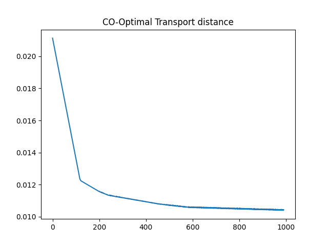
The first method requires learning the sample marginal distribution which minimizes the CO-Optimal Transport distance [49] between two input spaces. More precisely, given a source data \((X, \mu_x^{(s)}, \mu_x^{(f)})\) and a target matrix \(Y\) associated with a fixed histogram on features \(\mu_y^{(f)}\), we want to solve the following problem
where \(\Delta\) is the probability simplex. This minimization is done with a
simple projected gradient descent in PyTorch. We use the automatic backend of POT that
allows us to compute the CO-Optimal Transport distance with ot.coot.co_optimal_transport2()
with differentiable losses.
The second method simply requires direct application of unbalanced Co-Optimal Transport [71]. More precisely, it is enough to use the sample and feature coupling from solving
where all the marginal distributions are uniform.
# Author: Remi Flamary <remi.flamary@unice.fr>
#         Quang Huy Tran <quang-huy.tran@univ-ubs.fr>
# License: MIT License

# sphinx_gallery_thumbnail_number = 4

from matplotlib.patches import ConnectionPatch
import torch
import numpy as np

import matplotlib.pyplot as pl
import ot

from ot.coot import co_optimal_transport as coot
from ot.coot import co_optimal_transport2 as coot2
from ot.gromov._unbalanced import unbalanced_co_optimal_transport
Generate data
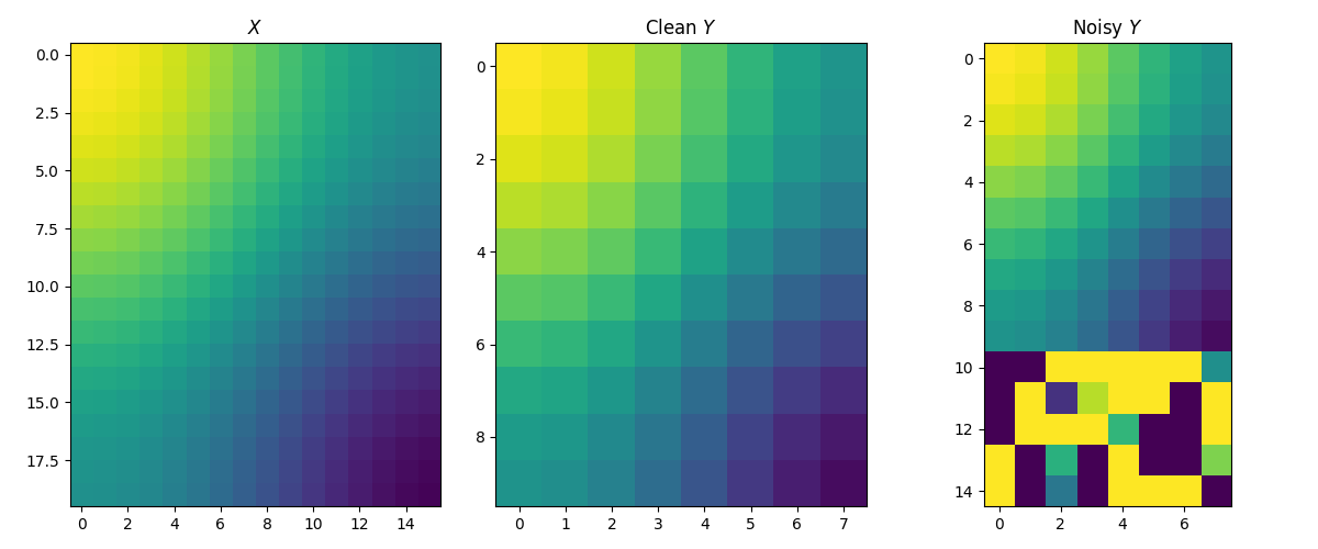
The source and clean target matrices are generated by \(X_{i,j} = \cos(\frac{i}{n_1} \pi) + \cos(\frac{j}{d_1} \pi)\) and \(Y_{i,j} = \cos(\frac{i}{n_2} \pi) + \cos(\frac{j}{d_2} \pi)\). The target matrix is then contaminated by adding 5 row outliers. Intuitively, we expect that the estimated sample distribution should ignore these outliers, i.e. their weights should be zero.
np.random.seed(182)

n1, d1 = 20, 16
n2, d2 = 10, 8
n = 15

X = (
    torch.cos(torch.arange(n1) * torch.pi / n1)[:, None]
    + torch.cos(torch.arange(d1) * torch.pi / d1)[None, :]
)

# Generate clean target data mixed with outliers
Y_noisy = torch.randn((n, d2)) * 10.0
Y_noisy[:n2, :] = (
    torch.cos(torch.arange(n2) * torch.pi / n2)[:, None]
    + torch.cos(torch.arange(d2) * torch.pi / d2)[None, :]
)
Y = Y_noisy[:n2, :]

X, Y_noisy, Y = X.double(), Y_noisy.double(), Y.double()

fig, axes = pl.subplots(nrows=1, ncols=3, figsize=(12, 5))
axes[0].imshow(X, vmin=-2, vmax=2)
axes[0].set_title("$X$")

axes[1].imshow(Y, vmin=-2, vmax=2)
axes[1].set_title("Clean $Y$")

axes[2].imshow(Y_noisy, vmin=-2, vmax=2)
axes[2].set_title("Noisy $Y$")

pl.tight_layout()

Optimize the COOT distance with respect to the sample marginal distribution
losses = []
lr = 1e-3
niter = 1000

b = torch.tensor(ot.unif(n), requires_grad=True)

for i in range(niter):
    loss = coot2(X, Y_noisy, wy_samp=b, log=False, verbose=False)
    losses.append(float(loss))

    loss.backward()

    with torch.no_grad():
        b -= lr * b.grad  # gradient step
        b[:] = ot.utils.proj_simplex(b)  # projection on the simplex

    b.grad.zero_()

# Estimated sample marginal distribution and training loss curve
pl.plot(losses[10:])
pl.title("CO-Optimal Transport distance")

print(f"Marginal distribution = {b.detach().numpy()}")

Marginal distribution = [0.07507868 0.08001347 0.09469872 0.1001999  0.10001527 0.10001687
 0.09999904 0.09979829 0.11466591 0.13551386 0.         0.
 0.         0.         0.        ]
Visualizing the row and column alignments with the estimated sample marginal distribution
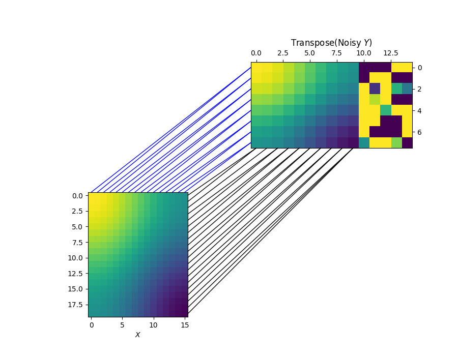
Clearly, the learned marginal distribution completely and successfully ignores the 5 outliers.
X, Y_noisy = X.numpy(), Y_noisy.numpy()
b = b.detach().numpy()

pi_sample, pi_feature = coot(X, Y_noisy, wy_samp=b, log=False, verbose=True)

fig = pl.figure(4, (9, 7))
pl.clf()

ax1 = pl.subplot(2, 2, 3)
pl.imshow(X, vmin=-2, vmax=2)
pl.xlabel("$X$")

ax2 = pl.subplot(2, 2, 2)
ax2.yaxis.tick_right()
pl.imshow(np.transpose(Y_noisy), vmin=-2, vmax=2)
pl.title("Transpose(Noisy $Y$)")
ax2.xaxis.tick_top()

for i in range(n1):
    j = np.argmax(pi_sample[i, :])
    xyA = (d1 - 0.5, i)
    xyB = (j, d2 - 0.5)
    con = ConnectionPatch(
        xyA=xyA, xyB=xyB, coordsA=ax1.transData, coordsB=ax2.transData, color="black"
    )
    fig.add_artist(con)

for i in range(d1):
    j = np.argmax(pi_feature[i, :])
    xyA = (i, -0.5)
    xyB = (-0.5, j)
    con = ConnectionPatch(
        xyA=xyA, xyB=xyB, coordsA=ax1.transData, coordsB=ax2.transData, color="blue"
    )
    fig.add_artist(con)

CO-Optimal Transport cost at iteration 1: 0.010389716046318456
Now, let see if we can use unbalanced Co-Optimal Transport to recover the clean OT plans, without the need of learning the marginal distribution as in Co-Optimal Transport. —————————————————————————————–
pi_sample, pi_feature = unbalanced_co_optimal_transport(
    X=X,
    Y=Y_noisy,
    reg_marginals=(10, 10),
    epsilon=0,
    divergence="kl",
    unbalanced_solver="mm",
    max_iter=1000,
    tol=1e-6,
    max_iter_ot=1000,
    tol_ot=1e-6,
    log=False,
    verbose=False,
)
Visualizing the row and column alignments learned by unbalanced Co-Optimal Transport.
Similar to Co-Optimal Transport, we are also be able to fully recover the clean OT plans.
fig = pl.figure(4, (9, 7))
pl.clf()

ax1 = pl.subplot(2, 2, 3)
pl.imshow(X, vmin=-2, vmax=2)
pl.xlabel("$X$")

ax2 = pl.subplot(2, 2, 2)
ax2.yaxis.tick_right()
pl.imshow(np.transpose(Y_noisy), vmin=-2, vmax=2)
pl.title("Transpose(Noisy $Y$)")
ax2.xaxis.tick_top()

for i in range(n1):
    j = np.argmax(pi_sample[i, :])
    xyA = (d1 - 0.5, i)
    xyB = (j, d2 - 0.5)
    con = ConnectionPatch(
        xyA=xyA, xyB=xyB, coordsA=ax1.transData, coordsB=ax2.transData, color="black"
    )
    fig.add_artist(con)

for i in range(d1):
    j = np.argmax(pi_feature[i, :])
    xyA = (i, -0.5)
    xyB = (-0.5, j)
    con = ConnectionPatch(
        xyA=xyA, xyB=xyB, coordsA=ax1.transData, coordsB=ax2.transData, color="blue"
    )
    fig.add_artist(con)

Total running time of the script: (0 minutes 5.245 seconds)