ot.mapping

Optimal Transport maps and variants

Warning

Note that by default the module is not imported in ot. In order to use it you need to explicitly import ot.mapping

Functions

ot.mapping.joint_OT_mapping_kernel(xs, xt, mu=1, eta=0.001, kerneltype='gaussian', sigma=1, bias=False, verbose=False, verbose2=False, numItermax=100, numInnerItermax=10, stopInnerThr=1e-06, stopThr=1e-05, log=False, **kwargs)

Joint OT and nonlinear mapping estimation with kernels as proposed in [8].

The function solves the following optimization problem:

\[ \begin{align}\begin{aligned}\min_{\gamma, L\in\mathcal{H}}\quad \|L(\mathbf{X_s}) - n_s\gamma \mathbf{X_t}\|^2_F + \mu \langle \gamma, \mathbf{M} \rangle_F + \eta \|L\|^2_\mathcal{H}\\s.t. \ \gamma \mathbf{1} = \mathbf{a}\\ \gamma^T \mathbf{1} = \mathbf{b}\\ \gamma \geq 0\end{aligned}\end{align} \]

where :

• \(\mathbf{M}\) is the (ns, nt) squared euclidean cost matrix between samples in \(\mathbf{X_s}\) and \(\mathbf{X_t}\) (scaled by \(n_s\))

• \(L\) is a \(n_s \times d\) linear operator on a kernel matrix that approximates the barycentric mapping

• \(\mathbf{a}\) and \(\mathbf{b}\) are uniform source and target weights

The problem consist in solving jointly an optimal transport matrix \(\gamma\) and the nonlinear mapping that fits the barycentric mapping \(n_s\gamma \mathbf{X_t}\).

One can also estimate a mapping with constant bias (see supplementary material of [8]) using the bias optional argument.

The algorithm used for solving the problem is the block coordinate descent that alternates between updates of \(\mathbf{G}\) (using conditional gradient) and the update of \(\mathbf{L}\) using a classical kernel least square solver.

Parameters:

• xs (array-like (ns,d)) – samples in the source domain

• xt (array-like (nt,d)) – samples in the target domain

• mu (float,optional) – Weight for the linear OT loss (>0)

• eta (float, optional) – Regularization term for the linear mapping L (>0)

• kerneltype (str,optional) – kernel used by calling function ot.utils.kernel() (gaussian by default)

• sigma (float, optional) – Gaussian kernel bandwidth.

• bias (bool,optional) – Estimate linear mapping with constant bias

• verbose (bool, optional) – Print information along iterations

• verbose2 (bool, optional) – Print information along iterations

• numItermax (int, optional) – Max number of BCD iterations

• numInnerItermax (int, optional) – Max number of iterations (inner CG solver)

• stopInnerThr (float, optional) – Stop threshold on error (inner CG solver) (>0)

• stopThr (float, optional) – Stop threshold on relative loss decrease (>0)

• log (bool, optional) – record log if True

Returns:

• gamma ((ns, nt) array-like) – Optimal transportation matrix for the given parameters

• L ((ns, d) array-like) – Nonlinear mapping matrix ((\(n_s+1\), d) if bias)

• log (dict) – log dictionary return only if log==True in parameters

References

[8]

M. Perrot, N. Courty, R. Flamary, A. Habrard, “Mapping estimation for discrete optimal transport”, Neural Information Processing Systems (NIPS), 2016.

See also

ot.lp.emd

Unregularized OT

ot.optim.cg

General regularized OT

ot.mapping.joint_OT_mapping_linear(xs, xt, mu=1, eta=0.001, bias=False, verbose=False, verbose2=False, numItermax=100, numInnerItermax=10, stopInnerThr=1e-06, stopThr=1e-05, log=False, **kwargs)

Joint OT and linear mapping estimation as proposed in [8].

The function solves the following optimization problem:

\[ \begin{align}\begin{aligned}\min_{\gamma,L}\quad \|L(\mathbf{X_s}) - n_s\gamma \mathbf{X_t} \|^2_F + \mu \langle \gamma, \mathbf{M} \rangle_F + \eta \|L - \mathbf{I}\|^2_F\\s.t. \ \gamma \mathbf{1} = \mathbf{a}\\ \gamma^T \mathbf{1} = \mathbf{b}\\ \gamma \geq 0\end{aligned}\end{align} \]

where :

• \(\mathbf{M}\) is the (ns, nt) squared euclidean cost matrix between samples in \(\mathbf{X_s}\) and \(\mathbf{X_t}\) (scaled by \(n_s\))

• \(L\) is a \(d\times d\) linear operator that approximates the barycentric mapping

• \(\mathbf{I}\) is the identity matrix (neutral linear mapping)

• \(\mathbf{a}\) and \(\mathbf{b}\) are uniform source and target weights

The problem consist in solving jointly an optimal transport matrix \(\gamma\) and a linear mapping that fits the barycentric mapping \(n_s\gamma \mathbf{X_t}\).

One can also estimate a mapping with constant bias (see supplementary material of [8]) using the bias optional argument.

The algorithm used for solving the problem is the block coordinate descent that alternates between updates of \(\mathbf{G}\) (using conditional gradient) and the update of \(\mathbf{L}\) using a classical least square solver.

Parameters:

• xs (array-like (ns,d)) – samples in the source domain

• xt (array-like (nt,d)) – samples in the target domain

• mu (float,optional) – Weight for the linear OT loss (>0)

• eta (float, optional) – Regularization term for the linear mapping L (>0)

• bias (bool,optional) – Estimate linear mapping with constant bias

• numItermax (int, optional) – Max number of BCD iterations

• stopThr (float, optional) – Stop threshold on relative loss decrease (>0)

• numInnerItermax (int, optional) – Max number of iterations (inner CG solver)

• stopInnerThr (float, optional) – Stop threshold on error (inner CG solver) (>0)

• verbose (bool, optional) – Print information along iterations

• log (bool, optional) – record log if True

Returns:

• gamma ((ns, nt) array-like) – Optimal transportation matrix for the given parameters

• L ((d, d) array-like) – Linear mapping matrix ((\(d+1\), d) if bias)

• log (dict) – log dictionary return only if log==True in parameters

References

[8]

M. Perrot, N. Courty, R. Flamary, A. Habrard, “Mapping estimation for discrete optimal transport”, Neural Information Processing Systems (NIPS), 2016.

See also

ot.lp.emd

Unregularized OT

ot.optim.cg

General regularized OT

ot.mapping.nearest_brenier_potential_fit(X, V, X_classes=None, a=None, b=None, strongly_convex_constant=0.6, gradient_lipschitz_constant=1.4, its=100, log=False, init_method='barycentric')

Computes optimal values and gradients at X for a strongly convex potential \(\varphi\) with Lipschitz gradients on the partitions defined by X_classes, where \(\varphi\) is optimal such that \(\nabla \varphi \#\mu \approx \nu\), given samples \(X = x_1, \cdots, x_n \sim \mu\) and \(V = v_1, \cdots, v_n \sim \nu\). Finding such a potential that has the desired regularity on the partition \((E_k)_{k \in [K]}\) (given by the classes X_classes) is equivalent to finding optimal values phi for the \(\varphi(x_i)\) and its gradients \(\nabla \varphi(x_i)\) (variable`G`). In practice, these optimal values are found by solving the following problem

\begin{gather*} \text{min} \sum_{i,j}\pi_{i,j}\|g_i - v_j\|_2^2 \\ g_1,\cdots, g_n \in \mathbb{R}^d,\; \varphi_1, \cdots, \varphi_n \in \mathbb{R},\; \pi \in \Pi(a, b) \\ \text{s.t.}\ \forall k \in [K],\; \forall i,j \in I_k: \\ \varphi_i-\varphi_j-\langle g_j, x_i-x_j\rangle \geq c_1\|g_i - g_j\|_2^2 + c_2\|x_i-x_j\|_2^2 - c_3\langle g_j-g_i, x_j -x_i \rangle. \end{gather*}

The constants \(c_1, c_2, c_3\) only depend on strongly_convex_constant and gradient_lipschitz_constant. The constraint \(\pi \in \Pi(a, b)\) denotes the fact that the matrix \(\pi\) belong to the OT polytope of marginals a and b. \(I_k\) is the subset of \([n]\) of the i such that \(x_i\) is in the partition (or class) \(E_k\), i.e. X_classes[i] == k.

This problem is solved by alternating over the variable \(\pi\) and the variables \(\varphi_i, g_i\). For \(\pi\), the problem is the standard discrete OT problem, and for \(\varphi_i, g_i\), the problem is a convex QCQP solved using cvxpy (ECOS solver).

Accepts any compatible backend, but will perform the QCQP optimisation on Numpy arrays, and convert back at the end.

Warning

This function requires the CVXPY library

Warning

Accepts any backend but will convert to Numpy then back to the backend.

Parameters:

• X (array-like (n, d)) – reference points used to compute the optimal values phi and G

• V (array-like (n, d)) – values of the gradients at the reference points X

• X_classes (array-like (n,), optional) – classes of the reference points, defaults to a single class

• a (array-like (n,), optional) – weights for the reference points X, defaults to uniform

• b (array-like (n,), optional) – weights for the target points V, defaults to uniform

• strongly_convex_constant (float, optional) – constant for the strong convexity of the input potential phi, defaults to 0.6

• gradient_lipschitz_constant (float, optional) – constant for the Lipschitz property of the input gradient G, defaults to 1.4

• its (int, optional) – number of iterations, defaults to 100

• log (bool, optional) – record log if true

• init_method (str, optional) – ‘target’ initialises G=V, ‘barycentric’ initialises at the image of X by the barycentric projection

Returns:

• phi (array-like (n,)) – optimal values of the potential at the points X

• G (array-like (n, d)) – optimal values of the gradients at the points X

• log (dict, optional) – If input log is true, a dictionary containing the values of the variables at each iteration, as well as solver information

References

[58]

François-Pierre Paty, Alexandre d’Aspremont, and Marco Cuturi. Regularity as regularization: Smooth and strongly convex brenier potentials in optimal transport. In International Conference on Artificial Intelligence and Statistics, pages 1222–1232. PMLR, 2020.

See also

ot.mapping.nearest_brenier_potential_predict_bounds

Predicting SSNB images on new source data

ot.da.NearestBrenierPotential

BaseTransport wrapper for SSNB

Examples using ot.mapping.nearest_brenier_potential_fit

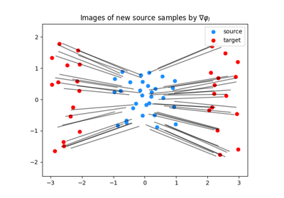
Smooth and Strongly Convex Nearest Brenier Potentials

Smooth and Strongly Convex Nearest Brenier Potentials

ot.mapping.nearest_brenier_potential_predict_bounds(X, phi, G, Y, X_classes=None, Y_classes=None, strongly_convex_constant=0.6, gradient_lipschitz_constant=1.4, log=False)

Compute the values of the lower and upper bounding potentials at the input points Y, using the potential optimal values phi at X and their gradients G at X. The ‘lower’ potential corresponds to the method from [58], Equation 2, while the bounding property and ‘upper’ potential come from [59], Theorem 3.14 (taking into account the fact that this theorem’s statement has a min instead of a max, which is a typo). Both potentials are optimal for the SSNB problem.

If \(I_k\) is the subset of \([n]\) of the i such that \(x_i\) is in the partition (or class) \(E_k\), for each \(y \in E_k\), this function solves the convex QCQP problems, respectively for l: ‘lower’ and u: ‘upper’:

\begin{gather*} (\varphi_{l}(x), \nabla \varphi_l(x)) = \text{argmin}\ t, \\ t\in \mathbb{R},\; g\in \mathbb{R}^d, \\ \text{s.t.} \forall j \in I_k,\; t-\varphi_j - \langle g_j, y-x_j \rangle \geq c_1\|g - g_j\|_2^2 + c_2\|y-x_j\|_2^2 - c_3\langle g_j-g, x_j -y \rangle. \end{gather*}

\begin{gather*} (\varphi_{u}(x), \nabla \varphi_u(x)) = \text{argmax}\ t, \\ t\in \mathbb{R},\; g\in \mathbb{R}^d, \\ \text{s.t.} \forall i \in I_k,\; \varphi_i^* -t - \langle g, x_i-y \rangle \geq c_1\|g_i - g\|_2^2 + c_2\|x_i-y\|_2^2 - c_3\langle g-g_i, y -x_i \rangle. \end{gather*}

The constants \(c_1, c_2, c_3\) only depend on strongly_convex_constant and gradient_lipschitz_constant.

Warning

This function requires the CVXPY library

Warning

Accepts any backend but will convert to Numpy then back to the backend.

Parameters:

• X (array-like (n, d)) – reference points used to compute the optimal values phi and G

• X_classes (array-like (n,), optional) – classes of the reference points

• phi (array-like (n,)) – optimal values of the potential at the points X

• G (array-like (n, d)) – optimal values of the gradients at the points X

• Y (array-like (m, d)) – input points

• X_classes – classes of the reference points, defaults to a single class

• Y_classes (array_like (m,), optional) – classes of the input points, defaults to a single class

• strongly_convex_constant (float, optional) – constant for the strong convexity of the input potential phi, defaults to 0.6

• gradient_lipschitz_constant (float, optional) – constant for the Lipschitz property of the input gradient G, defaults to 1.4

• log (bool, optional) – record log if true

Returns:

• phi_lu (array-like (2, m)) – values of the lower and upper bounding potentials at Y

• G_lu (array-like (2, m, d)) – gradients of the lower and upper bounding potentials at Y

• log (dict, optional) – If input log is true, a dictionary containing solver information

References

[58]

François-Pierre Paty, Alexandre d’Aspremont, and Marco Cuturi. Regularity as regularization: Smooth and strongly convex brenier potentials in optimal transport. In International Conference on Artificial Intelligence and Statistics, pages 1222–1232. PMLR, 2020.

[59]

Adrien B Taylor. Convex interpolation and performance estimation of first-order methods for convex optimization. PhD thesis, Catholic University of Louvain, Louvain-la-Neuve, Belgium, 2017.

See also

ot.mapping.nearest_brenier_potential_fit

Fitting the SSNB on source and target data

ot.da.NearestBrenierPotential

BaseTransport wrapper for SSNB

Examples using ot.mapping.nearest_brenier_potential_predict_bounds

Smooth and Strongly Convex Nearest Brenier Potentials

Smooth and Strongly Convex Nearest Brenier Potentials

ot.mapping.joint_OT_mapping_kernel(xs, xt, mu=1, eta=0.001, kerneltype='gaussian', sigma=1, bias=False, verbose=False, verbose2=False, numItermax=100, numInnerItermax=10, stopInnerThr=1e-06, stopThr=1e-05, log=False, **kwargs)

Joint OT and nonlinear mapping estimation with kernels as proposed in [8].

The function solves the following optimization problem:

\[ \begin{align}\begin{aligned}\min_{\gamma, L\in\mathcal{H}}\quad \|L(\mathbf{X_s}) - n_s\gamma \mathbf{X_t}\|^2_F + \mu \langle \gamma, \mathbf{M} \rangle_F + \eta \|L\|^2_\mathcal{H}\\s.t. \ \gamma \mathbf{1} = \mathbf{a}\\ \gamma^T \mathbf{1} = \mathbf{b}\\ \gamma \geq 0\end{aligned}\end{align} \]

where :

• \(\mathbf{M}\) is the (ns, nt) squared euclidean cost matrix between samples in \(\mathbf{X_s}\) and \(\mathbf{X_t}\) (scaled by \(n_s\))

• \(L\) is a \(n_s \times d\) linear operator on a kernel matrix that approximates the barycentric mapping

• \(\mathbf{a}\) and \(\mathbf{b}\) are uniform source and target weights

The problem consist in solving jointly an optimal transport matrix \(\gamma\) and the nonlinear mapping that fits the barycentric mapping \(n_s\gamma \mathbf{X_t}\).

One can also estimate a mapping with constant bias (see supplementary material of [8]) using the bias optional argument.

The algorithm used for solving the problem is the block coordinate descent that alternates between updates of \(\mathbf{G}\) (using conditional gradient) and the update of \(\mathbf{L}\) using a classical kernel least square solver.

Parameters:

• xs (array-like (ns,d)) – samples in the source domain

• xt (array-like (nt,d)) – samples in the target domain

• mu (float,optional) – Weight for the linear OT loss (>0)

• eta (float, optional) – Regularization term for the linear mapping L (>0)

• kerneltype (str,optional) – kernel used by calling function ot.utils.kernel() (gaussian by default)

• sigma (float, optional) – Gaussian kernel bandwidth.

• bias (bool,optional) – Estimate linear mapping with constant bias

• verbose (bool, optional) – Print information along iterations

• verbose2 (bool, optional) – Print information along iterations

• numItermax (int, optional) – Max number of BCD iterations

• numInnerItermax (int, optional) – Max number of iterations (inner CG solver)

• stopInnerThr (float, optional) – Stop threshold on error (inner CG solver) (>0)

• stopThr (float, optional) – Stop threshold on relative loss decrease (>0)

• log (bool, optional) – record log if True

Returns:

• gamma ((ns, nt) array-like) – Optimal transportation matrix for the given parameters

• L ((ns, d) array-like) – Nonlinear mapping matrix ((\(n_s+1\), d) if bias)

• log (dict) – log dictionary return only if log==True in parameters

References

[8]

M. Perrot, N. Courty, R. Flamary, A. Habrard, “Mapping estimation for discrete optimal transport”, Neural Information Processing Systems (NIPS), 2016.

See also

ot.lp.emd

Unregularized OT

ot.optim.cg

General regularized OT

ot.mapping.joint_OT_mapping_linear(xs, xt, mu=1, eta=0.001, bias=False, verbose=False, verbose2=False, numItermax=100, numInnerItermax=10, stopInnerThr=1e-06, stopThr=1e-05, log=False, **kwargs)

Joint OT and linear mapping estimation as proposed in [8].

The function solves the following optimization problem:

\[ \begin{align}\begin{aligned}\min_{\gamma,L}\quad \|L(\mathbf{X_s}) - n_s\gamma \mathbf{X_t} \|^2_F + \mu \langle \gamma, \mathbf{M} \rangle_F + \eta \|L - \mathbf{I}\|^2_F\\s.t. \ \gamma \mathbf{1} = \mathbf{a}\\ \gamma^T \mathbf{1} = \mathbf{b}\\ \gamma \geq 0\end{aligned}\end{align} \]

where :

• \(\mathbf{M}\) is the (ns, nt) squared euclidean cost matrix between samples in \(\mathbf{X_s}\) and \(\mathbf{X_t}\) (scaled by \(n_s\))

• \(L\) is a \(d\times d\) linear operator that approximates the barycentric mapping

• \(\mathbf{I}\) is the identity matrix (neutral linear mapping)

• \(\mathbf{a}\) and \(\mathbf{b}\) are uniform source and target weights

The problem consist in solving jointly an optimal transport matrix \(\gamma\) and a linear mapping that fits the barycentric mapping \(n_s\gamma \mathbf{X_t}\).

One can also estimate a mapping with constant bias (see supplementary material of [8]) using the bias optional argument.

The algorithm used for solving the problem is the block coordinate descent that alternates between updates of \(\mathbf{G}\) (using conditional gradient) and the update of \(\mathbf{L}\) using a classical least square solver.

Parameters:

• xs (array-like (ns,d)) – samples in the source domain

• xt (array-like (nt,d)) – samples in the target domain

• mu (float,optional) – Weight for the linear OT loss (>0)

• eta (float, optional) – Regularization term for the linear mapping L (>0)

• bias (bool,optional) – Estimate linear mapping with constant bias

• numItermax (int, optional) – Max number of BCD iterations

• stopThr (float, optional) – Stop threshold on relative loss decrease (>0)

• numInnerItermax (int, optional) – Max number of iterations (inner CG solver)

• stopInnerThr (float, optional) – Stop threshold on error (inner CG solver) (>0)

• verbose (bool, optional) – Print information along iterations

• log (bool, optional) – record log if True

Returns:

• gamma ((ns, nt) array-like) – Optimal transportation matrix for the given parameters

• L ((d, d) array-like) – Linear mapping matrix ((\(d+1\), d) if bias)

• log (dict) – log dictionary return only if log==True in parameters

References

[8]

M. Perrot, N. Courty, R. Flamary, A. Habrard, “Mapping estimation for discrete optimal transport”, Neural Information Processing Systems (NIPS), 2016.

See also

ot.lp.emd

Unregularized OT

ot.optim.cg

General regularized OT

ot.mapping.nearest_brenier_potential_fit(X, V, X_classes=None, a=None, b=None, strongly_convex_constant=0.6, gradient_lipschitz_constant=1.4, its=100, log=False, init_method='barycentric')

Computes optimal values and gradients at X for a strongly convex potential \(\varphi\) with Lipschitz gradients on the partitions defined by X_classes, where \(\varphi\) is optimal such that \(\nabla \varphi \#\mu \approx \nu\), given samples \(X = x_1, \cdots, x_n \sim \mu\) and \(V = v_1, \cdots, v_n \sim \nu\). Finding such a potential that has the desired regularity on the partition \((E_k)_{k \in [K]}\) (given by the classes X_classes) is equivalent to finding optimal values phi for the \(\varphi(x_i)\) and its gradients \(\nabla \varphi(x_i)\) (variable`G`). In practice, these optimal values are found by solving the following problem

\begin{gather*} \text{min} \sum_{i,j}\pi_{i,j}\|g_i - v_j\|_2^2 \\ g_1,\cdots, g_n \in \mathbb{R}^d,\; \varphi_1, \cdots, \varphi_n \in \mathbb{R},\; \pi \in \Pi(a, b) \\ \text{s.t.}\ \forall k \in [K],\; \forall i,j \in I_k: \\ \varphi_i-\varphi_j-\langle g_j, x_i-x_j\rangle \geq c_1\|g_i - g_j\|_2^2 + c_2\|x_i-x_j\|_2^2 - c_3\langle g_j-g_i, x_j -x_i \rangle. \end{gather*}

The constants \(c_1, c_2, c_3\) only depend on strongly_convex_constant and gradient_lipschitz_constant. The constraint \(\pi \in \Pi(a, b)\) denotes the fact that the matrix \(\pi\) belong to the OT polytope of marginals a and b. \(I_k\) is the subset of \([n]\) of the i such that \(x_i\) is in the partition (or class) \(E_k\), i.e. X_classes[i] == k.

This problem is solved by alternating over the variable \(\pi\) and the variables \(\varphi_i, g_i\). For \(\pi\), the problem is the standard discrete OT problem, and for \(\varphi_i, g_i\), the problem is a convex QCQP solved using cvxpy (ECOS solver).

Accepts any compatible backend, but will perform the QCQP optimisation on Numpy arrays, and convert back at the end.

Warning

This function requires the CVXPY library

Warning

Accepts any backend but will convert to Numpy then back to the backend.

Parameters:

• X (array-like (n, d)) – reference points used to compute the optimal values phi and G

• V (array-like (n, d)) – values of the gradients at the reference points X

• X_classes (array-like (n,), optional) – classes of the reference points, defaults to a single class

• a (array-like (n,), optional) – weights for the reference points X, defaults to uniform

• b (array-like (n,), optional) – weights for the target points V, defaults to uniform

• strongly_convex_constant (float, optional) – constant for the strong convexity of the input potential phi, defaults to 0.6

• gradient_lipschitz_constant (float, optional) – constant for the Lipschitz property of the input gradient G, defaults to 1.4

• its (int, optional) – number of iterations, defaults to 100

• log (bool, optional) – record log if true

• init_method (str, optional) – ‘target’ initialises G=V, ‘barycentric’ initialises at the image of X by the barycentric projection

Returns:

• phi (array-like (n,)) – optimal values of the potential at the points X

• G (array-like (n, d)) – optimal values of the gradients at the points X

• log (dict, optional) – If input log is true, a dictionary containing the values of the variables at each iteration, as well as solver information

References

[58]

François-Pierre Paty, Alexandre d’Aspremont, and Marco Cuturi. Regularity as regularization: Smooth and strongly convex brenier potentials in optimal transport. In International Conference on Artificial Intelligence and Statistics, pages 1222–1232. PMLR, 2020.

See also

ot.mapping.nearest_brenier_potential_predict_bounds

Predicting SSNB images on new source data

ot.da.NearestBrenierPotential

BaseTransport wrapper for SSNB

ot.mapping.nearest_brenier_potential_predict_bounds(X, phi, G, Y, X_classes=None, Y_classes=None, strongly_convex_constant=0.6, gradient_lipschitz_constant=1.4, log=False)

Compute the values of the lower and upper bounding potentials at the input points Y, using the potential optimal values phi at X and their gradients G at X. The ‘lower’ potential corresponds to the method from [58], Equation 2, while the bounding property and ‘upper’ potential come from [59], Theorem 3.14 (taking into account the fact that this theorem’s statement has a min instead of a max, which is a typo). Both potentials are optimal for the SSNB problem.

If \(I_k\) is the subset of \([n]\) of the i such that \(x_i\) is in the partition (or class) \(E_k\), for each \(y \in E_k\), this function solves the convex QCQP problems, respectively for l: ‘lower’ and u: ‘upper’:

\begin{gather*} (\varphi_{l}(x), \nabla \varphi_l(x)) = \text{argmin}\ t, \\ t\in \mathbb{R},\; g\in \mathbb{R}^d, \\ \text{s.t.} \forall j \in I_k,\; t-\varphi_j - \langle g_j, y-x_j \rangle \geq c_1\|g - g_j\|_2^2 + c_2\|y-x_j\|_2^2 - c_3\langle g_j-g, x_j -y \rangle. \end{gather*}

\begin{gather*} (\varphi_{u}(x), \nabla \varphi_u(x)) = \text{argmax}\ t, \\ t\in \mathbb{R},\; g\in \mathbb{R}^d, \\ \text{s.t.} \forall i \in I_k,\; \varphi_i^* -t - \langle g, x_i-y \rangle \geq c_1\|g_i - g\|_2^2 + c_2\|x_i-y\|_2^2 - c_3\langle g-g_i, y -x_i \rangle. \end{gather*}

The constants \(c_1, c_2, c_3\) only depend on strongly_convex_constant and gradient_lipschitz_constant.

Warning

This function requires the CVXPY library

Warning

Accepts any backend but will convert to Numpy then back to the backend.

Parameters:

• X (array-like (n, d)) – reference points used to compute the optimal values phi and G

• X_classes (array-like (n,), optional) – classes of the reference points

• phi (array-like (n,)) – optimal values of the potential at the points X

• G (array-like (n, d)) – optimal values of the gradients at the points X

• Y (array-like (m, d)) – input points

• X_classes – classes of the reference points, defaults to a single class

• Y_classes (array_like (m,), optional) – classes of the input points, defaults to a single class

• strongly_convex_constant (float, optional) – constant for the strong convexity of the input potential phi, defaults to 0.6

• gradient_lipschitz_constant (float, optional) – constant for the Lipschitz property of the input gradient G, defaults to 1.4

• log (bool, optional) – record log if true

Returns:

• phi_lu (array-like (2, m)) – values of the lower and upper bounding potentials at Y

• G_lu (array-like (2, m, d)) – gradients of the lower and upper bounding potentials at Y

• log (dict, optional) – If input log is true, a dictionary containing solver information

References

[58]

François-Pierre Paty, Alexandre d’Aspremont, and Marco Cuturi. Regularity as regularization: Smooth and strongly convex brenier potentials in optimal transport. In International Conference on Artificial Intelligence and Statistics, pages 1222–1232. PMLR, 2020.

[59]

Adrien B Taylor. Convex interpolation and performance estimation of first-order methods for convex optimization. PhD thesis, Catholic University of Louvain, Louvain-la-Neuve, Belgium, 2017.

See also

ot.mapping.nearest_brenier_potential_fit

Fitting the SSNB on source and target data

ot.da.NearestBrenierPotential

BaseTransport wrapper for SSNB