ot.regpath

Regularization path OT solvers

Functions

ot.regpath.complement_schur(M_current, b, d, id_pop)

This function computes the inverse of the design matrix in the regularization path using the Schur complement. Two cases may arise:

Case 1: one variable is added to the active set

\[\begin{split}M_{k+1}^{-1} = \begin{bmatrix} M_{k}^{-1} + s^{-1} M_{k}^{-1} \mathbf{b} \mathbf{b}^T M_{k}^{-1} \ & - M_{k}^{-1} \mathbf{b} s^{-1} \\ - s^{-1} \mathbf{b}^T M_{k}^{-1} & s^{-1} \end{bmatrix}\end{split}\]

where :

• \(M_k^{-1}\) is the inverse of the design matrix \(H_A^tH_A\) of the previous iteration

• \(\mathbf{b}\) is the last column of \(M_{k}\)

• \(s\) is the Schur complement, given by \(s = \mathbf{d} - \mathbf{b}^T M_{k}^{-1} \mathbf{b}\)

Case 2: one variable is removed from the active set.

\[M_{k+1}^{-1} = M^{-1}_{k \backslash q} - \frac{r_{-q,q} r^{T}_{-q,q}}{r_{q,q}}\]

where :

• \(q\) is the index of column and row to delete

• \(M^{-1}_{k \backslash q}\) is the previous inverse matrix deprived of the \(q\) th column and \(q\) th row

• \(r_{-q,q}\) is the \(q\) th column of \(M^{-1}_{k}\) without the \(q\) th element

• \(r_{q, q}\) is the element of \(q\) th column and \(q\) th row in \(M^{-1}_{k}\)

Parameters:

• M_current (ndarray, shape (size(A)-1, size(A)-1)) – Inverse matrix of \(H_A^tH_A\) at the previous iteration, with size(A) the size of the active set

• b (ndarray, shape (size(A)-1, )) – None for case 2 (removal), last column of \(M_{k}\) for case 1 (addition)

• d (float) – should be equal to 2 when UOT and 1 for the semi-relaxed OT

• id_pop (int) – Index of the variable to be removed, equal to -1 if no variable is deleted at the current iteration

Returns:

M – Inverse matrix of \(H_A^tH_A\) of the current iteration

Return type:

ndarray, shape (size(A), size(A))

References

[41]

Chapel, L., Flamary, R., Wu, H., Févotte, C., and Gasso, G. (2021). Unbalanced optimal transport through non-negative penalized linear regression. NeurIPS.

ot.regpath.compute_next_removal(phi, delta, current_gamma)

This function computes the next gamma value if a variable is removed at the next iteration of the regularization path.

We look for the largest value of the regularization parameter such that an element of the current solution vanishes

\[\max_{j \in A} \frac{\phi_j}{\delta_j}\]

where :

• A is the current active set

• \(\phi_j\) is the \(j\) th element of the intercept of the current solution

• \(\delta_j\) is the \(j\) th element of the slope of the current solution

Parameters:

• phi (ndarray, shape (size(A), )) – Intercept of the solution at the current iteration

• delta (ndarray, shape (size(A), )) – Slope of the solution at the current iteration

• current_gamma (float) – Value of the regularization parameter at the beginning of the current iteration

Returns:

• next_removal_gamma (float) – Gamma value if a variable is removed at the next iteration

• next_removal_index (int) – Index of the variable to be removed at the next iteration

References

[41]

Chapel, L., Flamary, R., Wu, H., Févotte, C., and Gasso, G. (2021). Unbalanced optimal transport through non-negative penalized linear regression. NeurIPS.

ot.regpath.compute_transport_plan(gamma, gamma_list, Pi_list)

Given the regularization path, this function computes the transport plan for any value of gamma thanks to the piecewise linearity of the path.

\[t(\gamma) = \phi(\gamma) - \gamma \delta(\gamma)\]

where:

• \(\gamma\) is the regularization parameter

• \(\phi(\gamma)\) is the corresponding intercept

• \(\delta(\gamma)\) is the corresponding slope

• \(\mathbf{t}\) is the flattened version of the transport matrix

Parameters:

• gamma (float) – Regularization coefficient

• gamma_list (list) – List of regularization parameters of the regularization path

• Pi_list (list) – List of all the solutions of the regularization path

Returns:

t – Vectorization of the transport plan corresponding to the given value of gamma

Return type:

np.ndarray (dim_a*dim_b, )

Examples

>>> import ot
>>> import numpy as np
>>> n = 3
>>> xs = np.array([1., 2., 3.]).reshape((n, 1))
>>> xt = np.array([5., 6., 7.]).reshape((n, 1))
>>> C = ot.dist(xs, xt)
>>> C /= C.max()
>>> a = np.array([0.2, 0.5, 0.3])
>>> b = np.array([0.2, 0.5, 0.3])
>>> t, pi_list, g_list = ot.regpath.regularization_path(a, b, C, reg=1e-4)
>>> gamma = 1
>>> t2 = ot.regpath.compute_transport_plan(gamma, g_list, pi_list)
>>> t2
array([0.        , 0.        , 0.        , 0.19722222, 0.05555556,
       0.        , 0.        , 0.24722222, 0.        ])

References

[41]

Chapel, L., Flamary, R., Wu, H., Févotte, C., and Gasso, G. (2021). Unbalanced optimal transport through non-negative penalized linear regression. NeurIPS.

Examples using ot.regpath.compute_transport_plan

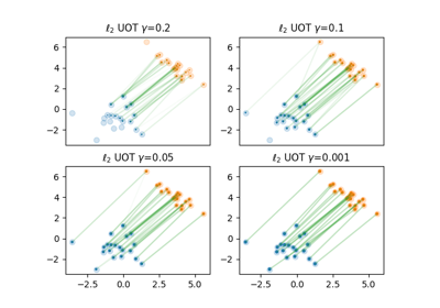
Regularization path of l2-penalized unbalanced optimal transport

Regularization path of l2-penalized unbalanced optimal transport

ot.regpath.construct_augmented_H(active_index, m, Hc, HrHr)

This function constructs an augmented matrix for the first iteration of the semi-relaxed regularization path

\[\begin{split}\text{Augmented}_H = \begin{bmatrix} 0 & H_{c A} \\ H_{c A}^T & H_{r A}^T H_{r A} \end{bmatrix}\end{split}\]

where :

• \(H_{r A}\) is the sub-matrix constructed by the columns of \(H_r\) whose indices belong to the active set A

• \(H_{c A}\) is the sub-matrix constructed by the columns of \(H_c\) whose indices belong to the active set A

Parameters:

• active_index (list) – Indices of the active variables

• m (int) – Length of the target distribution

• Hc (np.ndarray (dim_b, dim_a * dim_b)) – Matrix that computes the sum along the columns of the transport plan \(T\)

• HrHr (np.ndarray (dim_a * dim_b, dim_a * dim_b)) – Matrix product of \(H_r^T H_r\)

Returns:

H_augmented – Augmented matrix for the first iteration of the semi-relaxed regularization path

Return type:

np.ndarray (dim_b + size(A), dim_b + size(A))

ot.regpath.fully_relaxed_path(a: array, b: array, C: array, reg=0.0001, itmax=50000)

This function gives the regularization path of l2-penalized UOT problem

The problem to optimize is the Lasso reformulation of the l2-penalized UOT:

\[ \begin{align}\begin{aligned}\min_t \gamma \mathbf{c}^T \mathbf{t} + 0.5 * \|{H} \mathbf{t} - \mathbf{y}\|_2^2\\s.t. \mathbf{t} \geq 0\end{aligned}\end{align} \]

where :

• \(\mathbf{c}\) is the flattened version of the cost matrix \({C}\)

• \(\gamma = 1/\lambda\) is the l2-regularization coefficient

• \(\mathbf{y}\) is the concatenation of vectors \(\mathbf{a}\) and \(\mathbf{b}\), defined as \(\mathbf{y}^T = [\mathbf{a}^T \mathbf{b}^T]\)

• \({H}\) is a design matrix, see [41] for the design of \({H}\). The matrix product \(H\mathbf{t}\) computes both the source marginal and the target marginals.

• \(\mathbf{t}\) is the flattened version of the transport matrix

Parameters:

• a (np.ndarray (dim_a,)) – Histogram of dimension dim_a

• b (np.ndarray (dim_b,)) – Histogram of dimension dim_b

• C (np.ndarray, shape (dim_a, dim_b)) – Cost matrix

• reg (float) – l2-regularization coefficient

• itmax (int) – Maximum number of iteration

Returns:

• t (np.ndarray (dim_a*dim_b, )) – Flattened vector of the optimal transport matrix

• t_list (list) – List of solutions in the regularization path

• gamma_list (list) – List of regularization coefficients in the regularization path

Examples

>>> import ot
>>> import numpy as np
>>> n = 3
>>> xs = np.array([1., 2., 3.]).reshape((n, 1))
>>> xt = np.array([5., 6., 7.]).reshape((n, 1))
>>> C = ot.dist(xs, xt)
>>> C /= C.max()
>>> a = np.array([0.2, 0.5, 0.3])
>>> b = np.array([0.2, 0.5, 0.3])
>>> t, _, _ = ot.regpath.fully_relaxed_path(a, b, C, 1e-4)
>>> t
array([1.99958333e-01, 0.00000000e+00, 0.00000000e+00, 3.88888889e-05,
       4.99938889e-01, 0.00000000e+00, 0.00000000e+00, 3.88888889e-05,
       2.99958333e-01])

References

[41]

Chapel, L., Flamary, R., Wu, H., Févotte, C., and Gasso, G. (2021). Unbalanced optimal transport through non-negative penalized linear regression. NeurIPS.

ot.regpath.ot_next_gamma(phi, delta, HtH, Hty, c, active_index, current_gamma)

This function computes the next value of gamma if a variable is added in the next iteration of the regularization path.

We look for the largest value of gamma such that the gradient of an inactive variable vanishes

\[\max_{i \in \bar{A}} \frac{\mathbf{h}_i^T(H_A \phi - \mathbf{y})} {\mathbf{h}_i^T H_A \delta - \mathbf{c}_i}\]

where :

• A is the current active set

• \(\mathbf{h}_i\) is the \(i\) th column of the design matrix \({H}\)

• \({H}_A\) is the sub-matrix constructed by the columns of \({H}\) whose indices belong to the active set A

• \(\mathbf{c}_i\) is the \(i\) th element of the cost vector \(\mathbf{c}\)

• \(\mathbf{y}\) is the concatenation of the source and target distributions

• \(\phi\) is the intercept of the solutions at the current iteration

• \(\delta\) is the slope of the solutions at the current iteration

Parameters:

• phi (np.ndarray (size(A), )) – Intercept of the solutions at the current iteration

• delta (np.ndarray (size(A), )) – Slope of the solutions at the current iteration

• HtH (np.ndarray (dim_a * dim_b, dim_a * dim_b)) – Matrix product of \({H}^T {H}\)

• Hty (np.ndarray (dim_a + dim_b, )) – Matrix product of \({H}^T \mathbf{y}\)

• c (np.ndarray (dim_a * dim_b, )) – Flattened array of the cost matrix \({C}\)

• active_index (list) – Indices of active variables

• current_gamma (float) – Value of the regularization parameter at the beginning of the current iteration

Returns:

• next_gamma (float) – Value of gamma if a variable is added to active set in next iteration

• next_active_index (int) – Index of variable to be activated

References

[41]

Chapel, L., Flamary, R., Wu, H., Févotte, C., and Gasso, G. (2021). Unbalanced optimal transport through non-negative penalized linear regression. NeurIPS.

ot.regpath.recast_ot_as_lasso(a, b, C)

This function recasts the l2-penalized UOT problem as a Lasso problem.

Recall the l2-penalized UOT problem defined in [41]

\[ \begin{align}\begin{aligned}\text{UOT}_{\lambda} = \min_T <C, T> + \lambda \|T 1_m - \mathbf{a}\|_2^2 + \lambda \|T^T 1_n - \mathbf{b}\|_2^2\\s.t. T \geq 0\end{aligned}\end{align} \]

where :

• \(C\) is the cost matrix

• \(\lambda\) is the l2-regularization parameter

• \(\mathbf{a}\) and \(\mathbf{b}\) are the source and target distributions

• \(T\) is the transport plan to optimize

The problem above can be reformulated as a non-negative penalized linear regression problem, particularly Lasso

\[ \begin{align}\begin{aligned}\text{UOT2}_{\lambda} = \min_{\mathbf{t}} \gamma \mathbf{c}^T \mathbf{t} + 0.5 * \|H \mathbf{t} - \mathbf{y}\|_2^2\\s.t. \mathbf{t} \geq 0\end{aligned}\end{align} \]

where :

• \(\mathbf{c}\) is the flattened version of the cost matrix \(C\)

• \(\mathbf{y}\) is the concatenation of vectors \(\mathbf{a}\) and \(\mathbf{b}\)

• \(H\) is a metric matrix, see [41] for the design of \(H\). The matrix product \(H\mathbf{t}\) computes both the source marginal and the target marginals.

• \(\mathbf{t}\) is the flattened version of the transport plan \(T\)

Parameters:

• a (np.ndarray (dim_a,)) – Histogram of dimension dim_a

• b (np.ndarray (dim_b,)) – Histogram of dimension dim_b

• C (np.ndarray, shape (dim_a, dim_b)) – Cost matrix

Returns:

• H (np.ndarray (dim_a+dim_b, dim_a*dim_b)) – Design matrix that contains only 0 and 1

• y (np.ndarray (ns + nt, )) – Concatenation of histograms \(\mathbf{a}\) and \(\mathbf{b}\)

• c (np.ndarray (ns * nt, )) – Flattened array of the cost matrix

Examples

>>> import ot
>>> a = np.array([0.2, 0.3, 0.5])
>>> b = np.array([0.1, 0.9])
>>> C = np.array([[16., 25.], [28., 16.], [40., 36.]])
>>> H, y, c = ot.regpath.recast_ot_as_lasso(a, b, C)
>>> H.toarray()
array([[1., 1., 0., 0., 0., 0.],
       [0., 0., 1., 1., 0., 0.],
       [0., 0., 0., 0., 1., 1.],
       [1., 0., 1., 0., 1., 0.],
       [0., 1., 0., 1., 0., 1.]])
>>> y
array([0.2, 0.3, 0.5, 0.1, 0.9])
>>> c
array([16., 25., 28., 16., 40., 36.])

References

[41]

Chapel, L., Flamary, R., Wu, H., Févotte, C., and Gasso, G. (2021). Unbalanced optimal transport through non-negative penalized linear regression. NeurIPS.

ot.regpath.recast_semi_relaxed_as_lasso(a, b, C)

This function recasts the semi-relaxed l2-UOT problem as Lasso problem.

\[ \begin{align}\begin{aligned}\text{semi-relaxed UOT} = \min_T <C, T> + \lambda \|T 1_m - \mathbf{a}\|_2^2\\s.t. T^T 1_n = \mathbf{b}\\ \mathbf{t} \geq 0\end{aligned}\end{align} \]

where :

• \(C\) is the metric cost matrix

• \(\lambda\) is the l2-regularization parameter

• \(\mathbf{a}\) and \(\mathbf{b}\) are the source and target distributions

• \(T\) is the transport plan to optimize

The problem above can be reformulated as follows

\[ \begin{align}\begin{aligned}\text{semi-relaxed UOT2} = \min_t \gamma \mathbf{c}^T t + 0.5 * \|H_r \mathbf{t} - \mathbf{a}\|_2^2\\s.t. H_c \mathbf{t} = \mathbf{b}\\ \mathbf{t} \geq 0\end{aligned}\end{align} \]

where :

• \(\mathbf{c}\) is flattened version of the cost matrix \(C\)

• \(\gamma = 1/\lambda\) is the l2-regularization parameter

• \(H_r\) is a metric matrix which computes the sum along the rows of the transport plan \(T\)

• \(H_c\) is a metric matrix which computes the sum along the columns of the transport plan \(T\)

• \(\mathbf{t}\) is the flattened version of \(T\)

Parameters:

• a (np.ndarray (dim_a,)) – Histogram of dimension dim_a

• b (np.ndarray (dim_b,)) – Histogram of dimension dim_b

• C (np.ndarray, shape (dim_a, dim_b)) – Cost matrix

Returns:

• Hr (np.ndarray (dim_a, dim_a * dim_b)) – Auxiliary matrix constituted by 0 and 1, which computes the sum along the rows of transport plan \(T\)

• Hc (np.ndarray (dim_b, dim_a * dim_b)) – Auxiliary matrix constituted by 0 and 1, which computes the sum along the columns of transport plan \(T\)

• c (np.ndarray (ns * nt, )) – Flattened array of the cost matrix

Examples

>>> import ot
>>> a = np.array([0.2, 0.3, 0.5])
>>> b = np.array([0.1, 0.9])
>>> C = np.array([[16., 25.], [28., 16.], [40., 36.]])
>>> Hr,Hc,c = ot.regpath.recast_semi_relaxed_as_lasso(a, b, C)
>>> Hr.toarray()
array([[1., 1., 0., 0., 0., 0.],
       [0., 0., 1., 1., 0., 0.],
       [0., 0., 0., 0., 1., 1.]])
>>> Hc.toarray()
array([[1., 0., 1., 0., 1., 0.],
       [0., 1., 0., 1., 0., 1.]])
>>> c
array([16., 25., 28., 16., 40., 36.])

ot.regpath.regularization_path(a: array, b: array, C: array, reg=0.0001, semi_relaxed=False, itmax=50000)

This function provides all the solutions of the regularization path of the l2-UOT problem [41].

The problem to optimize is the Lasso reformulation of the l2-penalized UOT:

\[ \begin{align}\begin{aligned}\min_t \gamma \mathbf{c}^T \mathbf{t} + 0.5 * \|{H} \mathbf{t} - \mathbf{y}\|_2^2\\s.t. \mathbf{t} \geq 0\end{aligned}\end{align} \]

where :

• \(\mathbf{c}\) is the flattened version of the cost matrix \({C}\)

• \(\gamma = 1/\lambda\) is the l2-regularization coefficient

• \(\mathbf{y}\) is the concatenation of vectors \(\mathbf{a}\) and \(\mathbf{b}\), defined as \(\mathbf{y}^T = [\mathbf{a}^T \mathbf{b}^T]\)

• \({H}\) is a design matrix, see [41] for the design of \({H}\). The matrix product \(H\mathbf{t}\) computes both the source marginal and the target marginals.

• \(\mathbf{t}\) is the flattened version of the transport matrix

For the semi-relaxed problem, it optimizes the Lasso reformulation of the l2-penalized UOT:

\[ \begin{align}\begin{aligned}\min_t \gamma \mathbf{c}^T \mathbf{t} + 0.5 * \|H_r \mathbf{t} - \mathbf{a}\|_2^2\\s.t. H_c \mathbf{t} = \mathbf{b}\\ \mathbf{t} \geq 0\end{aligned}\end{align} \]

Parameters:

• a (np.ndarray (dim_a,)) – Histogram of dimension dim_a

• b (np.ndarray (dim_b,)) – Histogram of dimension dim_b

• C (np.ndarray, shape (dim_a, dim_b)) – Cost matrix

• reg (float (optional)) – l2-regularization coefficient

• semi_relaxed (bool (optional)) – Give the semi-relaxed path if True

• itmax (int (optional)) – Maximum number of iteration

Returns:

• t (np.ndarray (dim_a*dim_b, )) – Flattened vector of the (unregularized) optimal transport matrix

• t_list (list) – List of all the optimal transport vectors of the regularization path

• gamma_list (list) – List of the regularization parameters in the path

References

[41]

Chapel, L., Flamary, R., Wu, H., Févotte, C., and Gasso, G. (2021). Unbalanced optimal transport through non-negative penalized linear regression. NeurIPS.

Examples using ot.regpath.regularization_path

Regularization path of l2-penalized unbalanced optimal transport

Regularization path of l2-penalized unbalanced optimal transport

ot.regpath.semi_relaxed_next_gamma(phi, delta, phi_u, delta_u, HrHr, Hc, Hra, c, active_index, current_gamma)

This function computes the next value of gamma when a variable is active in the regularization path of semi-relaxed UOT.

By taking the Lagrangian form of the problem, we obtain a similar update as the two-sided relaxed UOT

\[\max_{i \in \bar{A}} \frac{\mathbf{h}_{ri}^T(H_{rA} \phi - \mathbf{a}) + \mathbf{h}_{c i}^T\phi_u}{\mathbf{h}_{r i}^T H_{r A} \delta + \ \mathbf{h}_{c i} \delta_u - \mathbf{c}_i}\]

where :

• A is the current active set

• \(\mathbf{h}_{r i}\) is the ith column of the matrix \(H_r\)

• \(\mathbf{h}_{c i}\) is the ith column of the matrix \(H_c\)

• \(H_{r A}\) is the sub-matrix constructed by the columns of \(H_r\) whose indices belong to the active set A

• \(\mathbf{c}_i\) is the \(i\) th element of cost vector \(\mathbf{c}\)

• \(\phi\) is the intercept of the solutions in current iteration

• \(\delta\) is the slope of the solutions in current iteration

• \(\phi_u\) is the intercept of Lagrange parameter at the current iteration

• \(\delta_u\) is the slope of Lagrange parameter at the current iteration

Parameters:

• phi (np.ndarray (size(A), )) – Intercept of the solutions at the current iteration

• delta (np.ndarray (size(A), )) – Slope of the solutions at the current iteration

• phi_u (np.ndarray (dim_b, )) – Intercept of the Lagrange parameter at the current iteration

• delta_u (np.ndarray (dim_b, )) – Slope of the Lagrange parameter at the current iteration

• HrHr (np.ndarray (dim_a * dim_b, dim_a * dim_b)) – Matrix product of \(H_r^T H_r\)

• Hc (np.ndarray (dim_b, dim_a * dim_b)) – Matrix that computes the sum along the columns of the transport plan \(T\)

• Hra (np.ndarray (dim_a * dim_b, )) – Matrix product of \(H_r^T \mathbf{a}\)

• c (np.ndarray (dim_a * dim_b, )) – Flattened array of cost matrix \(C\)

• active_index (list) – Indices of active variables

• current_gamma (float) – Value of regularization coefficient at the start of current iteration

Returns:

• next_gamma (float) – Value of gamma if a variable is added to active set in next iteration

• next_active_index (int) – Index of variable to be activated

References

[41]

Chapel, L., Flamary, R., Wu, H., Févotte, C., and Gasso, G. (2021). Unbalanced optimal transport through non-negative penalized linear regression. NeurIPS.

ot.regpath.semi_relaxed_path(a: array, b: array, C: array, reg=0.0001, itmax=50000)

This function gives the regularization path of semi-relaxed l2-UOT problem.

The problem to optimize is the Lasso reformulation of the l2-penalized UOT:

\[ \begin{align}\begin{aligned}\min_t \gamma \mathbf{c}^T t + 0.5 * \|H_r \mathbf{t} - \mathbf{a}\|_2^2\\s.t. H_c \mathbf{t} = \mathbf{b}\\ \mathbf{t} \geq 0\end{aligned}\end{align} \]

where :

• \(\mathbf{c}\) is the flattened version of the cost matrix \(C\)

• \(\gamma = 1/\lambda\) is the l2-regularization parameter

• \(H_r\) is a matrix that computes the sum along the rows of the transport plan \(T\)

• \(H_c\) is a matrix that computes the sum along the columns of the transport plan \(T\)

• \(\mathbf{t}\) is the flattened version of the transport plan \(T\)

Parameters:

• a (np.ndarray (dim_a,)) – Histogram of dimension dim_a

• b (np.ndarray (dim_b,)) – Histogram of dimension dim_b

• C (np.ndarray, shape (dim_a, dim_b)) – Cost matrix

• reg (float (optional)) – l2-regularization coefficient

• itmax (int (optional)) – Maximum number of iteration

Returns:

• t (np.ndarray (dim_a*dim_b, )) – Flattened vector of the (unregularized) optimal transport matrix

• t_list (list) – List of all the optimal transport vectors of the regularization path

• gamma_list (list) – List of the regularization parameters in the path

Examples

>>> import ot
>>> import numpy as np
>>> n = 3
>>> xs = np.array([1., 2., 3.]).reshape((n, 1))
>>> xt = np.array([5., 6., 7.]).reshape((n, 1))
>>> C = ot.dist(xs, xt)
>>> C /= C.max()
>>> a = np.array([0.2, 0.5, 0.3])
>>> b = np.array([0.2, 0.5, 0.3])
>>> t, _, _ = ot.regpath.semi_relaxed_path(a, b, C, 1e-4)
>>> t
array([1.99980556e-01, 0.00000000e+00, 0.00000000e+00, 1.94444444e-05,
       4.99980556e-01, 0.00000000e+00, 0.00000000e+00, 1.94444444e-05,
       3.00000000e-01])

References

[41]

Chapel, L., Flamary, R., Wu, H., Févotte, C., and Gasso, G. (2021). Unbalanced optimal transport through non-negative penalized linear regression. NeurIPS.

ot.regpath.complement_schur(M_current, b, d, id_pop)

This function computes the inverse of the design matrix in the regularization path using the Schur complement. Two cases may arise:

Case 1: one variable is added to the active set

\[\begin{split}M_{k+1}^{-1} = \begin{bmatrix} M_{k}^{-1} + s^{-1} M_{k}^{-1} \mathbf{b} \mathbf{b}^T M_{k}^{-1} \ & - M_{k}^{-1} \mathbf{b} s^{-1} \\ - s^{-1} \mathbf{b}^T M_{k}^{-1} & s^{-1} \end{bmatrix}\end{split}\]

where :

• \(M_k^{-1}\) is the inverse of the design matrix \(H_A^tH_A\) of the previous iteration

• \(\mathbf{b}\) is the last column of \(M_{k}\)

• \(s\) is the Schur complement, given by \(s = \mathbf{d} - \mathbf{b}^T M_{k}^{-1} \mathbf{b}\)

Case 2: one variable is removed from the active set.

\[M_{k+1}^{-1} = M^{-1}_{k \backslash q} - \frac{r_{-q,q} r^{T}_{-q,q}}{r_{q,q}}\]

where :

• \(q\) is the index of column and row to delete

• \(M^{-1}_{k \backslash q}\) is the previous inverse matrix deprived of the \(q\) th column and \(q\) th row

• \(r_{-q,q}\) is the \(q\) th column of \(M^{-1}_{k}\) without the \(q\) th element

• \(r_{q, q}\) is the element of \(q\) th column and \(q\) th row in \(M^{-1}_{k}\)

Parameters:

• M_current (ndarray, shape (size(A)-1, size(A)-1)) – Inverse matrix of \(H_A^tH_A\) at the previous iteration, with size(A) the size of the active set

• b (ndarray, shape (size(A)-1, )) – None for case 2 (removal), last column of \(M_{k}\) for case 1 (addition)

• d (float) – should be equal to 2 when UOT and 1 for the semi-relaxed OT

• id_pop (int) – Index of the variable to be removed, equal to -1 if no variable is deleted at the current iteration

Returns:

M – Inverse matrix of \(H_A^tH_A\) of the current iteration

Return type:

ndarray, shape (size(A), size(A))

References

[41]

Chapel, L., Flamary, R., Wu, H., Févotte, C., and Gasso, G. (2021). Unbalanced optimal transport through non-negative penalized linear regression. NeurIPS.

ot.regpath.compute_next_removal(phi, delta, current_gamma)

This function computes the next gamma value if a variable is removed at the next iteration of the regularization path.

We look for the largest value of the regularization parameter such that an element of the current solution vanishes

\[\max_{j \in A} \frac{\phi_j}{\delta_j}\]

where :

• A is the current active set

• \(\phi_j\) is the \(j\) th element of the intercept of the current solution

• \(\delta_j\) is the \(j\) th element of the slope of the current solution

Parameters:

• phi (ndarray, shape (size(A), )) – Intercept of the solution at the current iteration

• delta (ndarray, shape (size(A), )) – Slope of the solution at the current iteration

• current_gamma (float) – Value of the regularization parameter at the beginning of the current iteration

Returns:

• next_removal_gamma (float) – Gamma value if a variable is removed at the next iteration

• next_removal_index (int) – Index of the variable to be removed at the next iteration

References

[41]

Chapel, L., Flamary, R., Wu, H., Févotte, C., and Gasso, G. (2021). Unbalanced optimal transport through non-negative penalized linear regression. NeurIPS.

ot.regpath.compute_transport_plan(gamma, gamma_list, Pi_list)

Given the regularization path, this function computes the transport plan for any value of gamma thanks to the piecewise linearity of the path.

\[t(\gamma) = \phi(\gamma) - \gamma \delta(\gamma)\]

where:

• \(\gamma\) is the regularization parameter

• \(\phi(\gamma)\) is the corresponding intercept

• \(\delta(\gamma)\) is the corresponding slope

• \(\mathbf{t}\) is the flattened version of the transport matrix

Parameters:

• gamma (float) – Regularization coefficient

• gamma_list (list) – List of regularization parameters of the regularization path

• Pi_list (list) – List of all the solutions of the regularization path

Returns:

t – Vectorization of the transport plan corresponding to the given value of gamma

Return type:

np.ndarray (dim_a*dim_b, )

Examples

>>> import ot
>>> import numpy as np
>>> n = 3
>>> xs = np.array([1., 2., 3.]).reshape((n, 1))
>>> xt = np.array([5., 6., 7.]).reshape((n, 1))
>>> C = ot.dist(xs, xt)
>>> C /= C.max()
>>> a = np.array([0.2, 0.5, 0.3])
>>> b = np.array([0.2, 0.5, 0.3])
>>> t, pi_list, g_list = ot.regpath.regularization_path(a, b, C, reg=1e-4)
>>> gamma = 1
>>> t2 = ot.regpath.compute_transport_plan(gamma, g_list, pi_list)
>>> t2
array([0.        , 0.        , 0.        , 0.19722222, 0.05555556,
       0.        , 0.        , 0.24722222, 0.        ])

References

[41]

Chapel, L., Flamary, R., Wu, H., Févotte, C., and Gasso, G. (2021). Unbalanced optimal transport through non-negative penalized linear regression. NeurIPS.

ot.regpath.construct_augmented_H(active_index, m, Hc, HrHr)

This function constructs an augmented matrix for the first iteration of the semi-relaxed regularization path

\[\begin{split}\text{Augmented}_H = \begin{bmatrix} 0 & H_{c A} \\ H_{c A}^T & H_{r A}^T H_{r A} \end{bmatrix}\end{split}\]

where :

• \(H_{r A}\) is the sub-matrix constructed by the columns of \(H_r\) whose indices belong to the active set A

• \(H_{c A}\) is the sub-matrix constructed by the columns of \(H_c\) whose indices belong to the active set A

Parameters:

• active_index (list) – Indices of the active variables

• m (int) – Length of the target distribution

• Hc (np.ndarray (dim_b, dim_a * dim_b)) – Matrix that computes the sum along the columns of the transport plan \(T\)

• HrHr (np.ndarray (dim_a * dim_b, dim_a * dim_b)) – Matrix product of \(H_r^T H_r\)

Returns:

H_augmented – Augmented matrix for the first iteration of the semi-relaxed regularization path

Return type:

np.ndarray (dim_b + size(A), dim_b + size(A))

ot.regpath.fully_relaxed_path(a: array, b: array, C: array, reg=0.0001, itmax=50000)

This function gives the regularization path of l2-penalized UOT problem

The problem to optimize is the Lasso reformulation of the l2-penalized UOT:

\[ \begin{align}\begin{aligned}\min_t \gamma \mathbf{c}^T \mathbf{t} + 0.5 * \|{H} \mathbf{t} - \mathbf{y}\|_2^2\\s.t. \mathbf{t} \geq 0\end{aligned}\end{align} \]

where :

• \(\mathbf{c}\) is the flattened version of the cost matrix \({C}\)

• \(\gamma = 1/\lambda\) is the l2-regularization coefficient

• \(\mathbf{y}\) is the concatenation of vectors \(\mathbf{a}\) and \(\mathbf{b}\), defined as \(\mathbf{y}^T = [\mathbf{a}^T \mathbf{b}^T]\)

• \({H}\) is a design matrix, see [41] for the design of \({H}\). The matrix product \(H\mathbf{t}\) computes both the source marginal and the target marginals.

• \(\mathbf{t}\) is the flattened version of the transport matrix

Parameters:

• a (np.ndarray (dim_a,)) – Histogram of dimension dim_a

• b (np.ndarray (dim_b,)) – Histogram of dimension dim_b

• C (np.ndarray, shape (dim_a, dim_b)) – Cost matrix

• reg (float) – l2-regularization coefficient

• itmax (int) – Maximum number of iteration

Returns:

• t (np.ndarray (dim_a*dim_b, )) – Flattened vector of the optimal transport matrix

• t_list (list) – List of solutions in the regularization path

• gamma_list (list) – List of regularization coefficients in the regularization path

Examples

>>> import ot
>>> import numpy as np
>>> n = 3
>>> xs = np.array([1., 2., 3.]).reshape((n, 1))
>>> xt = np.array([5., 6., 7.]).reshape((n, 1))
>>> C = ot.dist(xs, xt)
>>> C /= C.max()
>>> a = np.array([0.2, 0.5, 0.3])
>>> b = np.array([0.2, 0.5, 0.3])
>>> t, _, _ = ot.regpath.fully_relaxed_path(a, b, C, 1e-4)
>>> t
array([1.99958333e-01, 0.00000000e+00, 0.00000000e+00, 3.88888889e-05,
       4.99938889e-01, 0.00000000e+00, 0.00000000e+00, 3.88888889e-05,
       2.99958333e-01])

References

[41]

Chapel, L., Flamary, R., Wu, H., Févotte, C., and Gasso, G. (2021). Unbalanced optimal transport through non-negative penalized linear regression. NeurIPS.

ot.regpath.ot_next_gamma(phi, delta, HtH, Hty, c, active_index, current_gamma)

This function computes the next value of gamma if a variable is added in the next iteration of the regularization path.

We look for the largest value of gamma such that the gradient of an inactive variable vanishes

\[\max_{i \in \bar{A}} \frac{\mathbf{h}_i^T(H_A \phi - \mathbf{y})} {\mathbf{h}_i^T H_A \delta - \mathbf{c}_i}\]

where :

• A is the current active set

• \(\mathbf{h}_i\) is the \(i\) th column of the design matrix \({H}\)

• \({H}_A\) is the sub-matrix constructed by the columns of \({H}\) whose indices belong to the active set A

• \(\mathbf{c}_i\) is the \(i\) th element of the cost vector \(\mathbf{c}\)

• \(\mathbf{y}\) is the concatenation of the source and target distributions

• \(\phi\) is the intercept of the solutions at the current iteration

• \(\delta\) is the slope of the solutions at the current iteration

Parameters:

• phi (np.ndarray (size(A), )) – Intercept of the solutions at the current iteration

• delta (np.ndarray (size(A), )) – Slope of the solutions at the current iteration

• HtH (np.ndarray (dim_a * dim_b, dim_a * dim_b)) – Matrix product of \({H}^T {H}\)

• Hty (np.ndarray (dim_a + dim_b, )) – Matrix product of \({H}^T \mathbf{y}\)

• c (np.ndarray (dim_a * dim_b, )) – Flattened array of the cost matrix \({C}\)

• active_index (list) – Indices of active variables

• current_gamma (float) – Value of the regularization parameter at the beginning of the current iteration

Returns:

• next_gamma (float) – Value of gamma if a variable is added to active set in next iteration

• next_active_index (int) – Index of variable to be activated

References

[41]

Chapel, L., Flamary, R., Wu, H., Févotte, C., and Gasso, G. (2021). Unbalanced optimal transport through non-negative penalized linear regression. NeurIPS.

ot.regpath.recast_ot_as_lasso(a, b, C)

This function recasts the l2-penalized UOT problem as a Lasso problem.

Recall the l2-penalized UOT problem defined in [41]

\[ \begin{align}\begin{aligned}\text{UOT}_{\lambda} = \min_T <C, T> + \lambda \|T 1_m - \mathbf{a}\|_2^2 + \lambda \|T^T 1_n - \mathbf{b}\|_2^2\\s.t. T \geq 0\end{aligned}\end{align} \]

where :

• \(C\) is the cost matrix

• \(\lambda\) is the l2-regularization parameter

• \(\mathbf{a}\) and \(\mathbf{b}\) are the source and target distributions

• \(T\) is the transport plan to optimize

The problem above can be reformulated as a non-negative penalized linear regression problem, particularly Lasso

\[ \begin{align}\begin{aligned}\text{UOT2}_{\lambda} = \min_{\mathbf{t}} \gamma \mathbf{c}^T \mathbf{t} + 0.5 * \|H \mathbf{t} - \mathbf{y}\|_2^2\\s.t. \mathbf{t} \geq 0\end{aligned}\end{align} \]

where :

• \(\mathbf{c}\) is the flattened version of the cost matrix \(C\)

• \(\mathbf{y}\) is the concatenation of vectors \(\mathbf{a}\) and \(\mathbf{b}\)

• \(H\) is a metric matrix, see [41] for the design of \(H\). The matrix product \(H\mathbf{t}\) computes both the source marginal and the target marginals.

• \(\mathbf{t}\) is the flattened version of the transport plan \(T\)

Parameters:

• a (np.ndarray (dim_a,)) – Histogram of dimension dim_a

• b (np.ndarray (dim_b,)) – Histogram of dimension dim_b

• C (np.ndarray, shape (dim_a, dim_b)) – Cost matrix

Returns:

• H (np.ndarray (dim_a+dim_b, dim_a*dim_b)) – Design matrix that contains only 0 and 1

• y (np.ndarray (ns + nt, )) – Concatenation of histograms \(\mathbf{a}\) and \(\mathbf{b}\)

• c (np.ndarray (ns * nt, )) – Flattened array of the cost matrix

Examples

>>> import ot
>>> a = np.array([0.2, 0.3, 0.5])
>>> b = np.array([0.1, 0.9])
>>> C = np.array([[16., 25.], [28., 16.], [40., 36.]])
>>> H, y, c = ot.regpath.recast_ot_as_lasso(a, b, C)
>>> H.toarray()
array([[1., 1., 0., 0., 0., 0.],
       [0., 0., 1., 1., 0., 0.],
       [0., 0., 0., 0., 1., 1.],
       [1., 0., 1., 0., 1., 0.],
       [0., 1., 0., 1., 0., 1.]])
>>> y
array([0.2, 0.3, 0.5, 0.1, 0.9])
>>> c
array([16., 25., 28., 16., 40., 36.])

References

[41]

Chapel, L., Flamary, R., Wu, H., Févotte, C., and Gasso, G. (2021). Unbalanced optimal transport through non-negative penalized linear regression. NeurIPS.

ot.regpath.recast_semi_relaxed_as_lasso(a, b, C)

This function recasts the semi-relaxed l2-UOT problem as Lasso problem.

\[ \begin{align}\begin{aligned}\text{semi-relaxed UOT} = \min_T <C, T> + \lambda \|T 1_m - \mathbf{a}\|_2^2\\s.t. T^T 1_n = \mathbf{b}\\ \mathbf{t} \geq 0\end{aligned}\end{align} \]

where :

• \(C\) is the metric cost matrix

• \(\lambda\) is the l2-regularization parameter

• \(\mathbf{a}\) and \(\mathbf{b}\) are the source and target distributions

• \(T\) is the transport plan to optimize

The problem above can be reformulated as follows

\[ \begin{align}\begin{aligned}\text{semi-relaxed UOT2} = \min_t \gamma \mathbf{c}^T t + 0.5 * \|H_r \mathbf{t} - \mathbf{a}\|_2^2\\s.t. H_c \mathbf{t} = \mathbf{b}\\ \mathbf{t} \geq 0\end{aligned}\end{align} \]

where :

• \(\mathbf{c}\) is flattened version of the cost matrix \(C\)

• \(\gamma = 1/\lambda\) is the l2-regularization parameter

• \(H_r\) is a metric matrix which computes the sum along the rows of the transport plan \(T\)

• \(H_c\) is a metric matrix which computes the sum along the columns of the transport plan \(T\)

• \(\mathbf{t}\) is the flattened version of \(T\)

Parameters:

• a (np.ndarray (dim_a,)) – Histogram of dimension dim_a

• b (np.ndarray (dim_b,)) – Histogram of dimension dim_b

• C (np.ndarray, shape (dim_a, dim_b)) – Cost matrix

Returns:

• Hr (np.ndarray (dim_a, dim_a * dim_b)) – Auxiliary matrix constituted by 0 and 1, which computes the sum along the rows of transport plan \(T\)

• Hc (np.ndarray (dim_b, dim_a * dim_b)) – Auxiliary matrix constituted by 0 and 1, which computes the sum along the columns of transport plan \(T\)

• c (np.ndarray (ns * nt, )) – Flattened array of the cost matrix

Examples

>>> import ot
>>> a = np.array([0.2, 0.3, 0.5])
>>> b = np.array([0.1, 0.9])
>>> C = np.array([[16., 25.], [28., 16.], [40., 36.]])
>>> Hr,Hc,c = ot.regpath.recast_semi_relaxed_as_lasso(a, b, C)
>>> Hr.toarray()
array([[1., 1., 0., 0., 0., 0.],
       [0., 0., 1., 1., 0., 0.],
       [0., 0., 0., 0., 1., 1.]])
>>> Hc.toarray()
array([[1., 0., 1., 0., 1., 0.],
       [0., 1., 0., 1., 0., 1.]])
>>> c
array([16., 25., 28., 16., 40., 36.])

ot.regpath.regularization_path(a: array, b: array, C: array, reg=0.0001, semi_relaxed=False, itmax=50000)

This function provides all the solutions of the regularization path of the l2-UOT problem [41].

The problem to optimize is the Lasso reformulation of the l2-penalized UOT:

\[ \begin{align}\begin{aligned}\min_t \gamma \mathbf{c}^T \mathbf{t} + 0.5 * \|{H} \mathbf{t} - \mathbf{y}\|_2^2\\s.t. \mathbf{t} \geq 0\end{aligned}\end{align} \]

where :

• \(\mathbf{c}\) is the flattened version of the cost matrix \({C}\)

• \(\gamma = 1/\lambda\) is the l2-regularization coefficient

• \(\mathbf{y}\) is the concatenation of vectors \(\mathbf{a}\) and \(\mathbf{b}\), defined as \(\mathbf{y}^T = [\mathbf{a}^T \mathbf{b}^T]\)

• \({H}\) is a design matrix, see [41] for the design of \({H}\). The matrix product \(H\mathbf{t}\) computes both the source marginal and the target marginals.

• \(\mathbf{t}\) is the flattened version of the transport matrix

For the semi-relaxed problem, it optimizes the Lasso reformulation of the l2-penalized UOT:

\[ \begin{align}\begin{aligned}\min_t \gamma \mathbf{c}^T \mathbf{t} + 0.5 * \|H_r \mathbf{t} - \mathbf{a}\|_2^2\\s.t. H_c \mathbf{t} = \mathbf{b}\\ \mathbf{t} \geq 0\end{aligned}\end{align} \]

Parameters:

• a (np.ndarray (dim_a,)) – Histogram of dimension dim_a

• b (np.ndarray (dim_b,)) – Histogram of dimension dim_b

• C (np.ndarray, shape (dim_a, dim_b)) – Cost matrix

• reg (float (optional)) – l2-regularization coefficient

• semi_relaxed (bool (optional)) – Give the semi-relaxed path if True

• itmax (int (optional)) – Maximum number of iteration

Returns:

• t (np.ndarray (dim_a*dim_b, )) – Flattened vector of the (unregularized) optimal transport matrix

• t_list (list) – List of all the optimal transport vectors of the regularization path

• gamma_list (list) – List of the regularization parameters in the path

References

[41]

Chapel, L., Flamary, R., Wu, H., Févotte, C., and Gasso, G. (2021). Unbalanced optimal transport through non-negative penalized linear regression. NeurIPS.

ot.regpath.semi_relaxed_next_gamma(phi, delta, phi_u, delta_u, HrHr, Hc, Hra, c, active_index, current_gamma)

This function computes the next value of gamma when a variable is active in the regularization path of semi-relaxed UOT.

By taking the Lagrangian form of the problem, we obtain a similar update as the two-sided relaxed UOT

\[\max_{i \in \bar{A}} \frac{\mathbf{h}_{ri}^T(H_{rA} \phi - \mathbf{a}) + \mathbf{h}_{c i}^T\phi_u}{\mathbf{h}_{r i}^T H_{r A} \delta + \ \mathbf{h}_{c i} \delta_u - \mathbf{c}_i}\]

where :

• A is the current active set

• \(\mathbf{h}_{r i}\) is the ith column of the matrix \(H_r\)

• \(\mathbf{h}_{c i}\) is the ith column of the matrix \(H_c\)

• \(H_{r A}\) is the sub-matrix constructed by the columns of \(H_r\) whose indices belong to the active set A

• \(\mathbf{c}_i\) is the \(i\) th element of cost vector \(\mathbf{c}\)

• \(\phi\) is the intercept of the solutions in current iteration

• \(\delta\) is the slope of the solutions in current iteration

• \(\phi_u\) is the intercept of Lagrange parameter at the current iteration

• \(\delta_u\) is the slope of Lagrange parameter at the current iteration

Parameters:

• phi (np.ndarray (size(A), )) – Intercept of the solutions at the current iteration

• delta (np.ndarray (size(A), )) – Slope of the solutions at the current iteration

• phi_u (np.ndarray (dim_b, )) – Intercept of the Lagrange parameter at the current iteration

• delta_u (np.ndarray (dim_b, )) – Slope of the Lagrange parameter at the current iteration

• HrHr (np.ndarray (dim_a * dim_b, dim_a * dim_b)) – Matrix product of \(H_r^T H_r\)

• Hc (np.ndarray (dim_b, dim_a * dim_b)) – Matrix that computes the sum along the columns of the transport plan \(T\)

• Hra (np.ndarray (dim_a * dim_b, )) – Matrix product of \(H_r^T \mathbf{a}\)

• c (np.ndarray (dim_a * dim_b, )) – Flattened array of cost matrix \(C\)

• active_index (list) – Indices of active variables

• current_gamma (float) – Value of regularization coefficient at the start of current iteration

Returns:

• next_gamma (float) – Value of gamma if a variable is added to active set in next iteration

• next_active_index (int) – Index of variable to be activated

References

[41]

Chapel, L., Flamary, R., Wu, H., Févotte, C., and Gasso, G. (2021). Unbalanced optimal transport through non-negative penalized linear regression. NeurIPS.

ot.regpath.semi_relaxed_path(a: array, b: array, C: array, reg=0.0001, itmax=50000)

This function gives the regularization path of semi-relaxed l2-UOT problem.

The problem to optimize is the Lasso reformulation of the l2-penalized UOT:

\[ \begin{align}\begin{aligned}\min_t \gamma \mathbf{c}^T t + 0.5 * \|H_r \mathbf{t} - \mathbf{a}\|_2^2\\s.t. H_c \mathbf{t} = \mathbf{b}\\ \mathbf{t} \geq 0\end{aligned}\end{align} \]

where :

• \(\mathbf{c}\) is the flattened version of the cost matrix \(C\)

• \(\gamma = 1/\lambda\) is the l2-regularization parameter

• \(H_r\) is a matrix that computes the sum along the rows of the transport plan \(T\)

• \(H_c\) is a matrix that computes the sum along the columns of the transport plan \(T\)

• \(\mathbf{t}\) is the flattened version of the transport plan \(T\)

Parameters:

• a (np.ndarray (dim_a,)) – Histogram of dimension dim_a

• b (np.ndarray (dim_b,)) – Histogram of dimension dim_b

• C (np.ndarray, shape (dim_a, dim_b)) – Cost matrix

• reg (float (optional)) – l2-regularization coefficient

• itmax (int (optional)) – Maximum number of iteration

Returns:

• t (np.ndarray (dim_a*dim_b, )) – Flattened vector of the (unregularized) optimal transport matrix

• t_list (list) – List of all the optimal transport vectors of the regularization path

• gamma_list (list) – List of the regularization parameters in the path

Examples

>>> import ot
>>> import numpy as np
>>> n = 3
>>> xs = np.array([1., 2., 3.]).reshape((n, 1))
>>> xt = np.array([5., 6., 7.]).reshape((n, 1))
>>> C = ot.dist(xs, xt)
>>> C /= C.max()
>>> a = np.array([0.2, 0.5, 0.3])
>>> b = np.array([0.2, 0.5, 0.3])
>>> t, _, _ = ot.regpath.semi_relaxed_path(a, b, C, 1e-4)
>>> t
array([1.99980556e-01, 0.00000000e+00, 0.00000000e+00, 1.94444444e-05,
       4.99980556e-01, 0.00000000e+00, 0.00000000e+00, 1.94444444e-05,
       3.00000000e-01])

References

[41]

Chapel, L., Flamary, R., Wu, H., Févotte, C., and Gasso, G. (2021). Unbalanced optimal transport through non-negative penalized linear regression. NeurIPS.