Wasserstein 1D (flow and barycenter) with PyTorch

In this small example, we consider the following minimization problem:

\[\mu^* = \min_\mu W(\mu,\nu)\]

where \(\nu\) is a reference 1D measure. The problem is handled by a projected gradient descent method, where the gradient is computed by pyTorch automatic differentiation. The projection on the simplex ensures that the iterate will remain on the probability simplex.

This example illustrates both wasserstein_1d function and backend use within the POT framework.

# Author: Nicolas Courty <ncourty@irisa.fr>
#         Rémi Flamary <remi.flamary@polytechnique.edu>
#
# License: MIT License

import numpy as np
import matplotlib.pylab as pl
import matplotlib as mpl
import torch

from ot.lp import wasserstein_1d
from ot.datasets import make_1D_gauss as gauss
from ot.utils import proj_simplex

red = np.array(mpl.colors.to_rgb('red'))
blue = np.array(mpl.colors.to_rgb('blue'))


n = 100  # nb bins

# bin positions
x = np.arange(n, dtype=np.float64)

# Gaussian distributions
a = gauss(n, m=20, s=5)  # m= mean, s= std
b = gauss(n, m=60, s=10)

# enforce sum to one on the support
a = a / a.sum()
b = b / b.sum()


device = "cuda" if torch.cuda.is_available() else "cpu"

# use pyTorch for our data
x_torch = torch.tensor(x).to(device=device)
a_torch = torch.tensor(a).to(device=device).requires_grad_(True)
b_torch = torch.tensor(b).to(device=device)

lr = 1e-6
nb_iter_max = 800

loss_iter = []

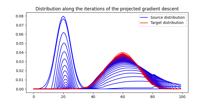
pl.figure(1, figsize=(8, 4))
pl.plot(x, a, 'b', label='Source distribution')
pl.plot(x, b, 'r', label='Target distribution')

for i in range(nb_iter_max):
    # Compute the Wasserstein 1D with torch backend
    loss = wasserstein_1d(x_torch, x_torch, a_torch, b_torch, p=2)
    # record the corresponding loss value
    loss_iter.append(loss.clone().detach().cpu().numpy())
    loss.backward()

    # performs a step of projected gradient descent
    with torch.no_grad():
        grad = a_torch.grad
        a_torch -= a_torch.grad * lr  # step
        a_torch.grad.zero_()
        a_torch.data = proj_simplex(a_torch)  # projection onto the simplex

    # plot one curve every 10 iterations
    if i % 10 == 0:
        mix = float(i) / nb_iter_max
        pl.plot(x, a_torch.clone().detach().cpu().numpy(), c=(1 - mix) * blue + mix * red)

pl.legend()
pl.title('Distribution along the iterations of the projected gradient descent')
pl.show()

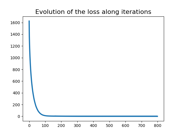
pl.figure(2)
pl.plot(range(nb_iter_max), loss_iter, lw=3)
pl.title('Evolution of the loss along iterations', fontsize=16)
pl.show()

• 
• 

/home/circleci/project/ot/lp/solver_1d.py:41: UserWarning: The use of `x.T` on tensors of dimension other than 2 to reverse their shape is deprecated and it will throw an error in a future release. Consider `x.mT` to transpose batches of matrices or `x.permute(*torch.arange(x.ndim - 1, -1, -1))` to reverse the dimensions of a tensor. (Triggered internally at ../aten/src/ATen/native/TensorShape.cpp:3614.)
  cws = cws.T.contiguous()

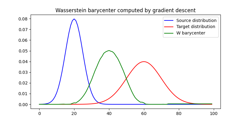
Wasserstein barycenter

In this example, we consider the following Wasserstein barycenter problem $$ \eta^* = \min_\eta;;; (1-t)W(\mu,\eta) + tW(\eta,\nu)$$ where \(\\mu\) and \(\\nu\) are reference 1D measures, and \(t\) is a parameter \(\in [0,1]\). The problem is handled by a project gradient descent method, where the gradient is computed by pyTorch automatic differentiation. The projection on the simplex ensures that the iterate will remain on the probability simplex.

This example illustrates both wasserstein_1d function and backend use within the POT framework.

device = "cuda" if torch.cuda.is_available() else "cpu"

# use pyTorch for our data
x_torch = torch.tensor(x).to(device=device)
a_torch = torch.tensor(a).to(device=device)
b_torch = torch.tensor(b).to(device=device)
bary_torch = torch.tensor((a + b).copy() / 2).to(device=device).requires_grad_(True)


lr = 1e-6
nb_iter_max = 2000

loss_iter = []

# instant of the interpolation
t = 0.5

for i in range(nb_iter_max):
    # Compute the Wasserstein 1D with torch backend
    loss = (1 - t) * wasserstein_1d(x_torch, x_torch, a_torch.detach(), bary_torch, p=2) + t * wasserstein_1d(x_torch, x_torch, b_torch, bary_torch, p=2)
    # record the corresponding loss value
    loss_iter.append(loss.clone().detach().cpu().numpy())
    loss.backward()

    # performs a step of projected gradient descent
    with torch.no_grad():
        grad = bary_torch.grad
        bary_torch -= bary_torch.grad * lr  # step
        bary_torch.grad.zero_()
        bary_torch.data = proj_simplex(bary_torch)  # projection onto the simplex

pl.figure(3, figsize=(8, 4))
pl.plot(x, a, 'b', label='Source distribution')
pl.plot(x, b, 'r', label='Target distribution')
pl.plot(x, bary_torch.clone().detach().cpu().numpy(), c='green', label='W barycenter')
pl.legend()
pl.title('Wasserstein barycenter computed by gradient descent')
pl.show()

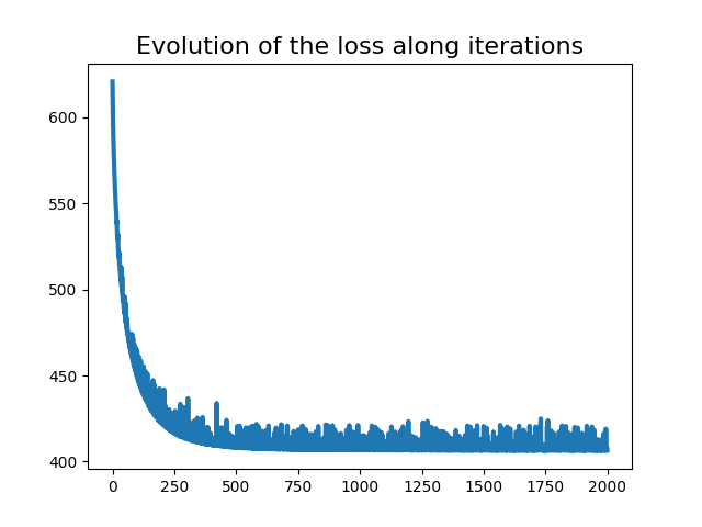
pl.figure(4)
pl.plot(range(nb_iter_max), loss_iter, lw=3)
pl.title('Evolution of the loss along iterations', fontsize=16)
pl.show()

• 
•