ot.plot
Functions for plotting OT matrices
Warning
Note that by default the module is not import in ot. In order to
use it you need to explicitly import ot.plot
Functions
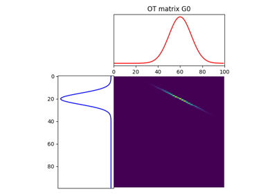
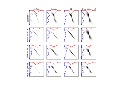
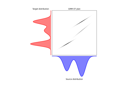
- ot.plot.plot1D_mat(a, b, M, title='', plot_style='yx', a_label='', b_label='', color_source='b', color_target='r', coupling_cmap='gray_r')[source]
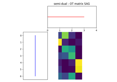
Plot matrix \(\mathbf{M}\) with the source and target 1D distributions.
Creates a subplot with the source distribution \(\mathbf{a}\) and target distribution \(\mathbf{b}\). In ‘yx’ mode (default), the source is on the left and the target on the top, and in ‘xy’ mode, source on the bottom (upside down) and the target on the left. The matrix \(\mathbf{M}\) is shown in between.
- Parameters:
a (ndarray, shape (na,)) – Source distribution
b (ndarray, shape (nb,)) – Target distribution
M (ndarray, shape (na, nb)) – Matrix to plot
title (str, optional) – Title of the plot
plot_style (str, optional) – Style of the plot, ‘yx’ or ‘xy’. ‘yx’ places the source on the left and the target on the top, ‘xy’ places the source on the bottom (upside down) and the target on the left.
a_label (str, optional) – Label for source distribution
b_label (str, optional) – Label for target distribution
color_source (str, optional) – Color of the source distribution
color_target (str, optional) – Color of the target distribution
coupling_cmap (str, optional) – Colormap for the coupling matrix
- Returns:
ax1 (source plot ax)
ax2 (target plot ax)
ax3 (coupling plot ax)
See also
Examples using ot.plot.plot1D_mat
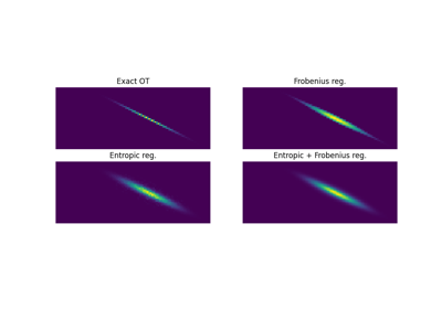
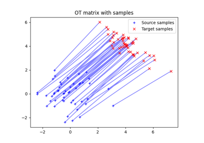
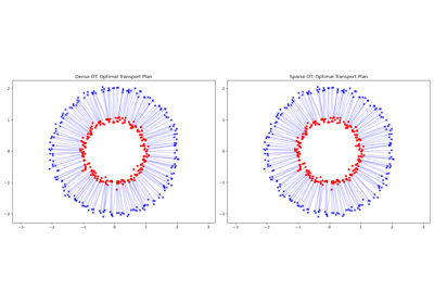
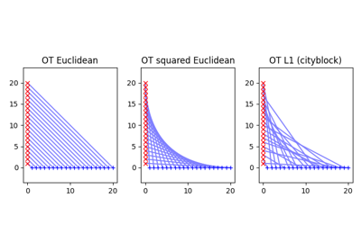
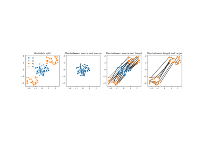
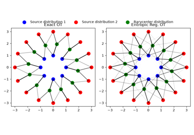
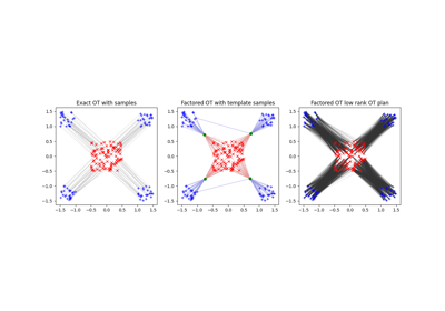
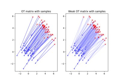
- ot.plot.plot2D_samples_mat(xs, xt, G, thr=1e-08, **kwargs)[source]
Plot matrix \(\mathbf{G}\) in 2D with lines using alpha values
Plot lines between source and target 2D samples with a color proportional to the value of the matrix \(\mathbf{G}\) between samples.
Supports both dense and sparse matrices. For sparse matrices, automatically detects the format and efficiently iterates only over non-zero entries.
- Parameters:
xs (ndarray, shape (ns,2)) – Source samples positions
xt (ndarray, shape (nt,2)) – Target samples positions
G (ndarray or sparse matrix, shape (ns,nt)) – OT matrix (dense array, scipy.sparse matrix, or backend array)
thr (float, optional) – threshold above which the line is drawn
**kwargs (dict) – parameters given to the plot functions (default color is black if nothing given)
Examples using ot.plot.plot2D_samples_mat
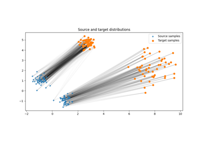
Dual OT solvers for entropic and quadratic regularized OT with Pytorch
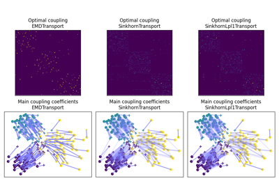
OT for domain adaptation on empirical distributions
- ot.plot.rescale_for_imshow_plot(x, y, n, m=None, a_y=None, b_y=None)[source]
Gives arrays xr, yr that can be plotted over an (n, m) imshow plot (in ‘xy’ coordinates). If a_y or b_y is provided, y is sliced over its indices such that y stays in [ay, by].
- Parameters:
- Returns:
xr (ndarray, shape (nx,)) – Rescaled x values (due to slicing, may have less elements than x)
yr (ndarray, shape (nx,)) – Rescaled y values (due to slicing, may have less elements than y)
See also
Examples using ot.plot.rescale_for_imshow_plot
- ot.plot.plot1D_mat(a, b, M, title='', plot_style='yx', a_label='', b_label='', color_source='b', color_target='r', coupling_cmap='gray_r')[source]
Plot matrix \(\mathbf{M}\) with the source and target 1D distributions.
Creates a subplot with the source distribution \(\mathbf{a}\) and target distribution \(\mathbf{b}\). In ‘yx’ mode (default), the source is on the left and the target on the top, and in ‘xy’ mode, source on the bottom (upside down) and the target on the left. The matrix \(\mathbf{M}\) is shown in between.
- Parameters:
a (ndarray, shape (na,)) – Source distribution
b (ndarray, shape (nb,)) – Target distribution
M (ndarray, shape (na, nb)) – Matrix to plot
title (str, optional) – Title of the plot
plot_style (str, optional) – Style of the plot, ‘yx’ or ‘xy’. ‘yx’ places the source on the left and the target on the top, ‘xy’ places the source on the bottom (upside down) and the target on the left.
a_label (str, optional) – Label for source distribution
b_label (str, optional) – Label for target distribution
color_source (str, optional) – Color of the source distribution
color_target (str, optional) – Color of the target distribution
coupling_cmap (str, optional) – Colormap for the coupling matrix
- Returns:
ax1 (source plot ax)
ax2 (target plot ax)
ax3 (coupling plot ax)
See also
- ot.plot.plot2D_samples_mat(xs, xt, G, thr=1e-08, **kwargs)[source]
Plot matrix \(\mathbf{G}\) in 2D with lines using alpha values
Plot lines between source and target 2D samples with a color proportional to the value of the matrix \(\mathbf{G}\) between samples.
Supports both dense and sparse matrices. For sparse matrices, automatically detects the format and efficiently iterates only over non-zero entries.
- Parameters:
xs (ndarray, shape (ns,2)) – Source samples positions
xt (ndarray, shape (nt,2)) – Target samples positions
G (ndarray or sparse matrix, shape (ns,nt)) – OT matrix (dense array, scipy.sparse matrix, or backend array)
thr (float, optional) – threshold above which the line is drawn
**kwargs (dict) – parameters given to the plot functions (default color is black if nothing given)
- ot.plot.rescale_for_imshow_plot(x, y, n, m=None, a_y=None, b_y=None)[source]
Gives arrays xr, yr that can be plotted over an (n, m) imshow plot (in ‘xy’ coordinates). If a_y or b_y is provided, y is sliced over its indices such that y stays in [ay, by].
- Parameters:
- Returns:
xr (ndarray, shape (nx,)) – Rescaled x values (due to slicing, may have less elements than x)
yr (ndarray, shape (nx,)) – Rescaled y values (due to slicing, may have less elements than y)
See also