Note
Go to the end to download the full example code.
Low rank Sinkhorn
This example illustrates the computation of Low Rank Sinkhorn [26].
[65] Scetbon, M., Cuturi, M., & Peyré, G. (2021). “Low-rank Sinkhorn factorization”. In International Conference on Machine Learning.
# Author: Laurène David <laurene.david@ip-paris.fr>
#
# License: MIT License
#
# sphinx_gallery_thumbnail_number = 2

import numpy as np
import matplotlib.pylab as pl
import ot.plot
from ot.datasets import make_1D_gauss as gauss
Generate data
n = 100
m = 120

# Gaussian distribution
a = gauss(n, m=int(n / 3), s=25 / np.sqrt(2)) + 1.5 * gauss(
    n, m=int(5 * n / 6), s=15 / np.sqrt(2)
)
a = a / np.sum(a)

b = 2 * gauss(m, m=int(m / 5), s=30 / np.sqrt(2)) + gauss(
    m, m=int(m / 2), s=35 / np.sqrt(2)
)
b = b / np.sum(b)

# Source and target distribution
X = np.arange(n).reshape(-1, 1)
Y = np.arange(m).reshape(-1, 1)
Solve Low rank sinkhorn
Solve low rank sinkhorn
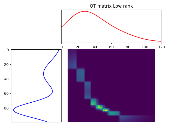
(<Axes: >, <Axes: >, <Axes: >)
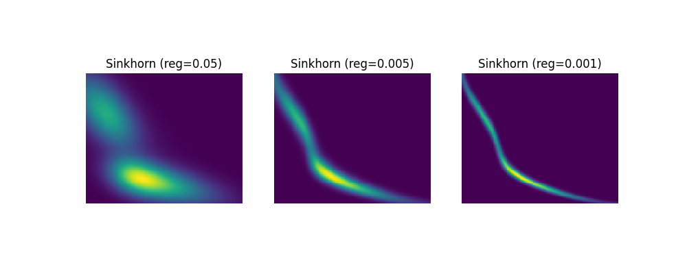
Sinkhorn vs Low Rank Sinkhorn
Compare Sinkhorn and Low rank sinkhorn with different regularizations and ranks.
/home/circleci/project/ot/lowrank.py:309: UserWarning: Dykstra did not converge. You might want to increase the number of iterations `numItermax`
  warnings.warn(
# Plot sinkhorn vs low rank sinkhorn
pl.figure(1, figsize=(10, 8))

pl.subplot(2, 3, 1)
pl.imshow(list_P_Sin[0], interpolation="nearest")
pl.axis("off")
pl.title("Sinkhorn (reg=0.05)")

pl.subplot(2, 3, 2)
pl.imshow(list_P_Sin[1], interpolation="nearest")
pl.axis("off")
pl.title("Sinkhorn (reg=0.005)")

pl.subplot(2, 3, 3)
pl.imshow(list_P_Sin[2], interpolation="nearest")
pl.axis("off")
pl.title("Sinkhorn (reg=0.001)")
pl.show()

pl.subplot(2, 3, 4)
pl.imshow(list_P_LR[0], interpolation="nearest")
pl.axis("off")
pl.title("Low rank (rank=3)")

pl.subplot(2, 3, 5)
pl.imshow(list_P_LR[1], interpolation="nearest")
pl.axis("off")
pl.title("Low rank (rank=10)")

pl.subplot(2, 3, 6)
pl.imshow(list_P_LR[2], interpolation="nearest")
pl.axis("off")
pl.title("Low rank (rank=50)")

pl.tight_layout()
Total running time of the script: (0 minutes 17.690 seconds)