Note
Go to the end to download the full example code.
Continuous OT plan estimation with Pytorch
Note
Example added in release: 0.8.2.
# Author: Remi Flamary <remi.flamary@polytechnique.edu>
#
# License: MIT License

# sphinx_gallery_thumbnail_number = 3

import numpy as np
import matplotlib.pyplot as pl
import torch
from torch import nn
import ot
import ot.plot
Data generation
torch.manual_seed(42)
np.random.seed(42)
n_source_samples = 1000
n_target_samples = 1000
theta = 2 * np.pi / 20
noise_level = 0.1
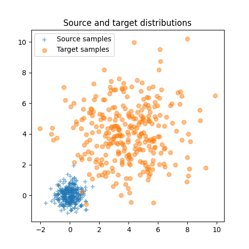
Xs = np.random.randn(n_source_samples, 2) * 0.5
Xt = np.random.randn(n_target_samples, 2) * 2
# one of the target mode changes its variance (no linear mapping)
Xt = Xt + 4
Plot data
nvisu = 300
pl.figure(1, (5, 5))
pl.clf()
pl.scatter(Xs[:nvisu, 0], Xs[:nvisu, 1], marker="+", label="Source samples", alpha=0.5)
pl.scatter(Xt[:nvisu, 0], Xt[:nvisu, 1], marker="o", label="Target samples", alpha=0.5)
pl.legend(loc=0)
ax_bounds = pl.axis()
pl.title("Source and target distributions")
Text(0.5, 1.0, 'Source and target distributions')
Convert data to torch tensors
xs = torch.tensor(Xs)
xt = torch.tensor(Xt)
Estimating deep dual variables for entropic OT
torch.manual_seed(42)

# define the MLP model


class Potential(torch.nn.Module):
    def __init__(self):
        super(Potential, self).__init__()
        self.fc1 = nn.Linear(2, 200)
        self.fc2 = nn.Linear(200, 1)
        self.relu = torch.nn.ReLU()  # instead of Heaviside step fn

    def forward(self, x):
        output = self.fc1(x)
        output = self.relu(output)  # instead of Heaviside step fn
        output = self.fc2(output)
        return output.ravel()


u = Potential().double()
v = Potential().double()

reg = 1

optimizer = torch.optim.Adam(list(u.parameters()) + list(v.parameters()), lr=0.005)

# number of iteration
n_iter = 500
n_batch = 500


losses = []

for i in range(n_iter):
    # generate noise samples

    iperms = torch.randint(0, n_source_samples, (n_batch,))
    ipermt = torch.randint(0, n_target_samples, (n_batch,))

    xsi = xs[iperms]
    xti = xt[ipermt]

    # minus because we maximize the dual loss
    loss = -ot.stochastic.loss_dual_entropic(u(xsi), v(xti), xsi, xti, reg=reg)
    losses.append(float(loss.detach()))

    if i % 10 == 0:
        print("Iter: {:3d}, loss={}".format(i, losses[-1]))

    loss.backward()
    optimizer.step()
    optimizer.zero_grad()


pl.figure(2)
pl.plot(losses)
pl.grid()
pl.title("Dual objective (negative)")
pl.xlabel("Iterations")
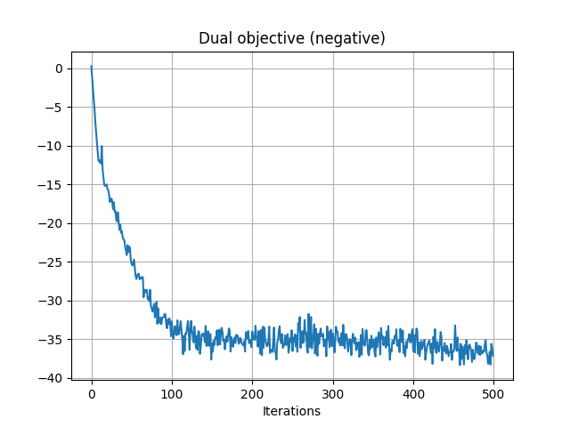
Iter:   0, loss=0.257329928299894
Iter:  10, loss=-11.890456785604675
Iter:  20, loss=-15.58037947236615
Iter:  30, loss=-18.440996850749865
Iter:  40, loss=-22.12608610815788
Iter:  50, loss=-25.27590340578239
Iter:  60, loss=-27.268827591939186
Iter:  70, loss=-29.79159074243252
Iter:  80, loss=-31.63488731570214
Iter:  90, loss=-32.127228618478725
Iter: 100, loss=-32.696522621311644
Iter: 110, loss=-33.46949401889149
Iter: 120, loss=-32.64206913098603
Iter: 130, loss=-36.153816351532946
Iter: 140, loss=-34.28321242161009
Iter: 150, loss=-35.520585380642636
Iter: 160, loss=-35.67609658732353
Iter: 170, loss=-34.45865441165184
Iter: 180, loss=-34.43596310348252
Iter: 190, loss=-35.261945704106836
Iter: 200, loss=-34.01278968196741
Iter: 210, loss=-36.87401169938976
Iter: 220, loss=-35.128205680449874
Iter: 230, loss=-37.63722430960618
Iter: 240, loss=-35.659266219020246
Iter: 250, loss=-36.527425475361845
Iter: 260, loss=-36.126583681704034
Iter: 270, loss=-31.735871196038296
Iter: 280, loss=-36.157560505651844
Iter: 290, loss=-35.070647347170436
Iter: 300, loss=-34.27069736487666
Iter: 310, loss=-35.4032555710632
Iter: 320, loss=-35.7515193321185
Iter: 330, loss=-35.505787072896766
Iter: 340, loss=-35.833572391120526
Iter: 350, loss=-35.540097202879465
Iter: 360, loss=-33.547154649280394
Iter: 370, loss=-35.635978662861795
Iter: 380, loss=-35.85734724064163
Iter: 390, loss=-37.221950448334646
Iter: 400, loss=-36.545262551431136
Iter: 410, loss=-35.202882711135615
Iter: 420, loss=-35.14673091868494
Iter: 430, loss=-35.32427691564021
Iter: 440, loss=-36.51095472212391
Iter: 450, loss=-36.56664149963812
Iter: 460, loss=-37.5571464161218
Iter: 470, loss=-35.7012331965002
Iter: 480, loss=-36.75436312339336
Iter: 490, loss=-35.12920968279601

Text(0.5, 23.633333333333333, 'Iterations')
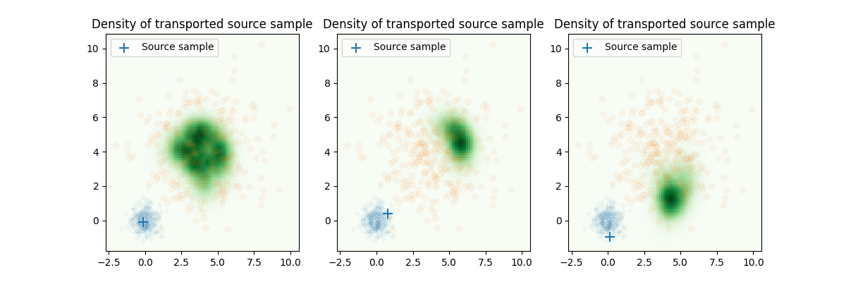
Plot the density on target for a given source sample
nv = 100
xl = np.linspace(ax_bounds[0], ax_bounds[1], nv)
yl = np.linspace(ax_bounds[2], ax_bounds[3], nv)

XX, YY = np.meshgrid(xl, yl)

xg = np.concatenate((XX.ravel()[:, None], YY.ravel()[:, None]), axis=1)

wxg = np.exp(-((xg[:, 0] - 4) ** 2 + (xg[:, 1] - 4) ** 2) / (2 * 2))
wxg = wxg / np.sum(wxg)

xg = torch.tensor(xg)
wxg = torch.tensor(wxg)


pl.figure(4, (12, 4))
pl.clf()
pl.subplot(1, 3, 1)

iv = 2
Gg = ot.stochastic.plan_dual_entropic(
    u(xs[iv : iv + 1, :]), v(xg), xs[iv : iv + 1, :], xg, reg=reg, wt=wxg
)
Gg = Gg.reshape((nv, nv)).detach().numpy()

pl.scatter(Xs[:nvisu, 0], Xs[:nvisu, 1], marker="+", zorder=2, alpha=0.05)
pl.scatter(Xt[:nvisu, 0], Xt[:nvisu, 1], marker="o", zorder=2, alpha=0.05)
pl.scatter(
    Xs[iv : iv + 1, 0],
    Xs[iv : iv + 1, 1],
    s=100,
    marker="+",
    label="Source sample",
    zorder=2,
    alpha=1,
    color="C0",
)
pl.pcolormesh(XX, YY, Gg, cmap="Greens", label="Density of transported source sample")
pl.legend(loc=0)
ax_bounds = pl.axis()
pl.title("Density of transported source sample")

pl.subplot(1, 3, 2)

iv = 3
Gg = ot.stochastic.plan_dual_entropic(
    u(xs[iv : iv + 1, :]), v(xg), xs[iv : iv + 1, :], xg, reg=reg, wt=wxg
)
Gg = Gg.reshape((nv, nv)).detach().numpy()

pl.scatter(Xs[:nvisu, 0], Xs[:nvisu, 1], marker="+", zorder=2, alpha=0.05)
pl.scatter(Xt[:nvisu, 0], Xt[:nvisu, 1], marker="o", zorder=2, alpha=0.05)
pl.scatter(
    Xs[iv : iv + 1, 0],
    Xs[iv : iv + 1, 1],
    s=100,
    marker="+",
    label="Source sample",
    zorder=2,
    alpha=1,
    color="C0",
)
pl.pcolormesh(XX, YY, Gg, cmap="Greens", label="Density of transported source sample")
pl.legend(loc=0)
ax_bounds = pl.axis()
pl.title("Density of transported source sample")

pl.subplot(1, 3, 3)

iv = 6
Gg = ot.stochastic.plan_dual_entropic(
    u(xs[iv : iv + 1, :]), v(xg), xs[iv : iv + 1, :], xg, reg=reg, wt=wxg
)
Gg = Gg.reshape((nv, nv)).detach().numpy()

pl.scatter(Xs[:nvisu, 0], Xs[:nvisu, 1], marker="+", zorder=2, alpha=0.05)
pl.scatter(Xt[:nvisu, 0], Xt[:nvisu, 1], marker="o", zorder=2, alpha=0.05)
pl.scatter(
    Xs[iv : iv + 1, 0],
    Xs[iv : iv + 1, 1],
    s=100,
    marker="+",
    label="Source sample",
    zorder=2,
    alpha=1,
    color="C0",
)
pl.pcolormesh(XX, YY, Gg, cmap="Greens", label="Density of transported source sample")
pl.legend(loc=0)
ax_bounds = pl.axis()
pl.title("Density of transported source sample")
/home/circleci/project/examples/backends/plot_stoch_continuous_ot_pytorch.py:171: UserWarning: Legend does not support handles for QuadMesh instances.
See: https://matplotlib.org/stable/tutorials/intermediate/legend_guide.html#implementing-a-custom-legend-handler
  pl.legend(loc=0)
/home/circleci/project/examples/backends/plot_stoch_continuous_ot_pytorch.py:196: UserWarning: Legend does not support handles for QuadMesh instances.
See: https://matplotlib.org/stable/tutorials/intermediate/legend_guide.html#implementing-a-custom-legend-handler
  pl.legend(loc=0)
/home/circleci/project/examples/backends/plot_stoch_continuous_ot_pytorch.py:221: UserWarning: Legend does not support handles for QuadMesh instances.
See: https://matplotlib.org/stable/tutorials/intermediate/legend_guide.html#implementing-a-custom-legend-handler
  pl.legend(loc=0)

Text(0.5, 1.0, 'Density of transported source sample')
Total running time of the script: (0 minutes 29.680 seconds)