ot.lp
Solvers for the original linear program OT problem.
Functions
- ot.lp.center_ot_dual(alpha0, beta0, a=None, b=None)[source]
Center dual OT potentials w.r.t. their weights
The main idea of this function is to find unique dual potentials that ensure some kind of centering/fairness. The main idea is to find dual potentials that lead to the same final objective value for both source and targets (see below for more details). It will help having stability when multiple calling of the OT solver with small changes.
Basically we add another constraint to the potential that will not change the objective value but will ensure unicity. The constraint is the following:
\[\alpha^T \mathbf{a} = \beta^T \mathbf{b}\]in addition to the OT problem constraints.
since \(\sum_i a_i=\sum_j b_j\) this can be solved by adding/removing a constant from both \(\alpha_0\) and \(\beta_0\).
\[ \begin{align}\begin{aligned}c &= \frac{\beta_0^T \mathbf{b} - \alpha_0^T \mathbf{a}}{\mathbf{1}^T \mathbf{b} + \mathbf{1}^T \mathbf{a}}\\\alpha &= \alpha_0 + c\\\beta &= \beta_0 + c\end{aligned}\end{align} \]- Parameters:
alpha0 ((ns,) numpy.ndarray, float64) – Source dual potential
beta0 ((nt,) numpy.ndarray, float64) – Target dual potential
a ((ns,) numpy.ndarray, float64) – Source histogram (uniform weight if empty list)
b ((nt,) numpy.ndarray, float64) – Target histogram (uniform weight if empty list)
- Returns:
alpha ((ns,) numpy.ndarray, float64) – Source centered dual potential
beta ((nt,) numpy.ndarray, float64) – Target centered dual potential
- ot.lp.check_number_threads(numThreads)[source]
Checks whether or not the requested number of threads has a valid value.
- ot.lp.emd(a, b, M, numItermax=100000, log=False, center_dual=True, numThreads=1, check_marginals=True)[source]
Solves the Earth Movers distance problem and returns the OT matrix
\[ \begin{align}\begin{aligned}\gamma = \mathop{\arg \min}_\gamma \quad \langle \gamma, \mathbf{M} \rangle_F\\s.t. \ \gamma \mathbf{1} = \mathbf{a}\\ \gamma^T \mathbf{1} = \mathbf{b}\\ \gamma \geq 0\end{aligned}\end{align} \]where :
\(\mathbf{M}\) is the metric cost matrix
\(\mathbf{a}\) and \(\mathbf{b}\) are the sample weights
Warning
Note that the \(\mathbf{M}\) matrix in numpy needs to be a C-order numpy.array in float64 format. It will be converted if not in this format
Note
This function is backend-compatible and will work on arrays from all compatible backends. But the algorithm uses the C++ CPU backend which can lead to copy overhead on GPU arrays.
Note
This function will cast the computed transport plan to the data type of the provided input with the following priority: \(\mathbf{a}\), then \(\mathbf{b}\), then \(\mathbf{M}\) if marginals are not provided. Casting to an integer tensor might result in a loss of precision. If this behaviour is unwanted, please make sure to provide a floating point input.
Note
An error will be raised if the vectors \(\mathbf{a}\) and \(\mathbf{b}\) do not sum to the same value.
Uses the algorithm proposed in [1].
- Parameters:
a ((ns,) array-like, float) – Source histogram (uniform weight if empty list)
b ((nt,) array-like, float) – Target histogram (uniform weight if empty list)
M ((ns,nt) array-like, float) – Loss matrix (c-order array in numpy with type float64)
numItermax (int, optional (default=100000)) – The maximum number of iterations before stopping the optimization algorithm if it has not converged.
log (bool, optional (default=False)) – If True, returns a dictionary containing the cost and dual variables. Otherwise returns only the optimal transportation matrix.
center_dual (boolean, optional (default=True)) – If True, centers the dual potential using function
ot.lp.center_ot_dual().numThreads (int or "max", optional (default=1, i.e. OpenMP is not used)) – If compiled with OpenMP, chooses the number of threads to parallelize. “max” selects the highest number possible.
check_marginals (bool, optional (default=True)) – If True, checks that the marginals mass are equal. If False, skips the check.
- Returns:
gamma (array-like, shape (ns, nt)) – Optimal transportation matrix for the given parameters
log (dict, optional) – If input log is true, a dictionary containing the cost and dual variables and exit status
Examples
Simple example with obvious solution. The function emd accepts lists and perform automatic conversion to numpy arrays
>>> import ot
>>> a=[.5,.5]
>>> b=[.5,.5]
>>> M=[[0.,1.],[1.,0.]]
>>> ot.emd(a, b, M)
array([[0.5, 0. ],
       [0. , 0.5]])
References
See also
ot.bregman.sinkhornEntropic regularized OT
ot.optim.cgGeneral regularized OT
- ot.lp.emd2(a, b, M, processes=1, numItermax=100000, log=False, return_matrix=False, center_dual=True, numThreads=1, check_marginals=True)[source]
Solves the Earth Movers distance problem and returns the loss
\[ \begin{align}\begin{aligned}\min_\gamma \quad \langle \gamma, \mathbf{M} \rangle_F\\s.t. \ \gamma \mathbf{1} = \mathbf{a}\\ \gamma^T \mathbf{1} = \mathbf{b}\\ \gamma \geq 0\end{aligned}\end{align} \]where :
\(\mathbf{M}\) is the metric cost matrix
\(\mathbf{a}\) and \(\mathbf{b}\) are the sample weights
Note
This function is backend-compatible and will work on arrays from all compatible backends. But the algorithm uses the C++ CPU backend which can lead to copy overhead on GPU arrays.
Note
This function will cast the computed transport plan and transportation loss to the data type of the provided input with the following priority: \(\mathbf{a}\), then \(\mathbf{b}\), then \(\mathbf{M}\) if marginals are not provided. Casting to an integer tensor might result in a loss of precision. If this behaviour is unwanted, please make sure to provide a floating point input.
Note
An error will be raised if the vectors \(\mathbf{a}\) and \(\mathbf{b}\) do not sum to the same value.
Uses the algorithm proposed in [1].
- Parameters:
a ((ns,) array-like, float64) – Source histogram (uniform weight if empty list)
b ((nt,) array-like, float64) – Target histogram (uniform weight if empty list)
M ((ns,nt) array-like, float64) – Loss matrix (for numpy c-order array with type float64)
processes (int, optional (default=1)) – Nb of processes used for multiple emd computation (deprecated)
numItermax (int, optional (default=100000)) – The maximum number of iterations before stopping the optimization algorithm if it has not converged.
log (boolean, optional (default=False)) – If True, returns a dictionary containing dual variables. Otherwise returns only the optimal transportation cost.
return_matrix (boolean, optional (default=False)) – If True, returns the optimal transportation matrix in the log.
center_dual (boolean, optional (default=True)) – If True, centers the dual potential using function
ot.lp.center_ot_dual().numThreads (int or "max", optional (default=1, i.e. OpenMP is not used)) – If compiled with OpenMP, chooses the number of threads to parallelize. “max” selects the highest number possible.
check_marginals (bool, optional (default=True)) – If True, checks that the marginals mass are equal. If False, skips the check.
- Returns:
W (float, array-like) – Optimal transportation loss for the given parameters
log (dict) – If input log is true, a dictionary containing dual variables and exit status
Examples
Simple example with obvious solution. The function emd accepts lists and perform automatic conversion to numpy arrays
>>> import ot
>>> a=[.5,.5]
>>> b=[.5,.5]
>>> M=[[0.,1.],[1.,0.]]
>>> ot.emd2(a,b,M)
0.0
References
See also
ot.bregman.sinkhornEntropic regularized OT
ot.optim.cgGeneral regularized OT
- ot.lp.estimate_dual_null_weights(alpha0, beta0, a, b, M)[source]
Estimate feasible values for 0-weighted dual potentials
The feasible values are computed efficiently but rather coarsely.
Warning
This function is necessary because the C++ solver in emd_c discards all samples in the distributions with zeros weights. This means that while the primal variable (transport matrix) is exact, the solver only returns feasible dual potentials on the samples with weights different from zero.
First we compute the constraints violations:
\[\mathbf{V} = \alpha + \beta^T - \mathbf{M}\]Next we compute the max amount of violation per row (\(\alpha\)) and columns (\(beta\))
\[ \begin{align}\begin{aligned}\mathbf{v^a}_i = \max_j \mathbf{V}_{i,j}\\\mathbf{v^b}_j = \max_i \mathbf{V}_{i,j}\end{aligned}\end{align} \]Finally we update the dual potential with 0 weights if a constraint is violated
\[ \begin{align}\begin{aligned}\alpha_i = \alpha_i - \mathbf{v^a}_i \quad \text{ if } \mathbf{a}_i=0 \text{ and } \mathbf{v^a}_i>0\\\beta_j = \beta_j - \mathbf{v^b}_j \quad \text{ if } \mathbf{b}_j=0 \text{ and } \mathbf{v^b}_j > 0\end{aligned}\end{align} \]In the end the dual potentials are centered using function
ot.lp.center_ot_dual().Note that all those updates do not change the objective value of the solution but provide dual potentials that do not violate the constraints.
- Parameters:
alpha0 ((ns,) numpy.ndarray, float64) – Source dual potential
beta0 ((nt,) numpy.ndarray, float64) – Target dual potential
alpha0 – Source dual potential
beta0 – Target dual potential
a ((ns,) numpy.ndarray, float64) – Source distribution (uniform weights if empty list)
b ((nt,) numpy.ndarray, float64) – Target distribution (uniform weights if empty list)
M ((ns,nt) numpy.ndarray, float64) – Loss matrix (c-order array with type float64)
- Returns:
alpha ((ns,) numpy.ndarray, float64) – Source corrected dual potential
beta ((nt,) numpy.ndarray, float64) – Target corrected dual potential
- ot.lp.free_support_barycenter(measures_locations, measures_weights, X_init, b=None, weights=None, numItermax=100, stopThr=1e-07, verbose=False, log=None, numThreads=1)[source]
Solves the free support (locations of the barycenters are optimized, not the weights) Wasserstein barycenter problem (i.e. the weighted Frechet mean for the 2-Wasserstein distance), formally:
\[\min_\mathbf{X} \quad \sum_{i=1}^N w_i W_2^2(\mathbf{b}, \mathbf{X}, \mathbf{a}_i, \mathbf{X}_i)\]where :
\(w \in \mathbb{(0, 1)}^{N}\)’s are the barycenter weights and sum to one
measure_weights denotes the \(\mathbf{a}_i \in \mathbb{R}^{k_i}\): empirical measures weights (on simplex)
measures_locations denotes the \(\mathbf{X}_i \in \mathbb{R}^{k_i, d}\): empirical measures atoms locations
\(\mathbf{b} \in \mathbb{R}^{k}\) is the desired weights vector of the barycenter
This problem is considered in [20] (Algorithm 2). There are two differences with the following codes:
we do not optimize over the weights
we do not do line search for the locations updates, we use i.e. \(\theta = 1\) in [20] (Algorithm 2). This can be seen as a discrete implementation of the fixed-point algorithm of [43] proposed in the continuous setting.
- Parameters:
measures_locations (list of N (k_i,d) array-like) – The discrete support of a measure supported on \(k_i\) locations of a d-dimensional space (\(k_i\) can be different for each element of the list)
measures_weights (list of N (k_i,) array-like) – Numpy arrays where each numpy array has \(k_i\) non-negatives values summing to one representing the weights of each discrete input measure
X_init ((k,d) array-like) – Initialization of the support locations (on k atoms) of the barycenter
b ((k,) array-like) – Initialization of the weights of the barycenter (non-negatives, sum to 1)
weights ((N,) array-like) – Initialization of the coefficients of the barycenter (non-negatives, sum to 1)
numItermax (int, optional) – Max number of iterations
stopThr (float, optional) – Stop threshold on error (>0)
verbose (bool, optional) – Print information along iterations
log (bool, optional) – record log if True
numThreads (int or "max", optional (default=1, i.e. OpenMP is not used)) – If compiled with OpenMP, chooses the number of threads to parallelize. “max” selects the highest number possible.
- Returns:
X – Support locations (on k atoms) of the barycenter
- Return type:
(k,d) array-like
References
Examples using ot.lp.free_support_barycenter
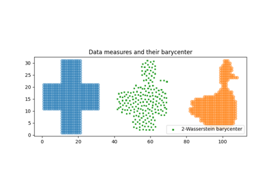
2D free support Wasserstein barycenters of distributions
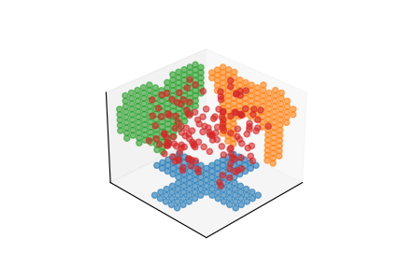
- ot.lp.generalized_free_support_barycenter(X_list, a_list, P_list, n_samples_bary, Y_init=None, b=None, weights=None, numItermax=100, stopThr=1e-07, verbose=False, log=None, numThreads=1, eps=0)[source]
Solves the free support generalized Wasserstein barycenter problem: finding a barycenter (a discrete measure with a fixed amount of points of uniform weights) whose respective projections fit the input measures. More formally:
\[\min_\gamma \quad \sum_{i=1}^p w_i W_2^2(\nu_i, \mathbf{P}_i\#\gamma)\]where :
\(\gamma = \sum_{l=1}^n b_l\delta_{y_l}\) is the desired barycenter with each \(y_l \in \mathbb{R}^d\)
\(\mathbf{b} \in \mathbb{R}^{n}\) is the desired weights vector of the barycenter
The input measures are \(\nu_i = \sum_{j=1}^{k_i}a_{i,j}\delta_{x_{i,j}}\)
The \(\mathbf{a}_i \in \mathbb{R}^{k_i}\) are the respective empirical measures weights (on the simplex)
The \(\mathbf{X}_i \in \mathbb{R}^{k_i, d_i}\) are the respective empirical measures atoms locations
\(w = (w_1, \cdots w_p)\) are the barycenter coefficients (on the simplex)
Each \(\mathbf{P}_i \in \mathbb{R}^{d, d_i}\), and \(P_i\#\nu_i = \sum_{j=1}^{k_i}a_{i,j}\delta_{P_ix_{i,j}}\)
As show by [42], this problem can be re-written as a Wasserstein Barycenter problem, which we solve using the free support method [20] (Algorithm 2).
- Parameters:
X_list (list of p (k_i,d_i) array-like) – Discrete supports of the input measures: each consists of \(k_i\) locations of a d_i-dimensional space (\(k_i\) can be different for each element of the list)
a_list (list of p (k_i,) array-like) – Measure weights: each element is a vector (k_i) on the simplex
P_list (list of p (d_i,d) array-like) – Each \(P_i\) is a linear map \(\mathbb{R}^{d} \rightarrow \mathbb{R}^{d_i}\)
n_samples_bary (int) – Number of barycenter points
Y_init ((n_samples_bary,d) array-like) – Initialization of the support locations (on k atoms) of the barycenter
b ((n_samples_bary,) array-like) – Initialization of the weights of the barycenter measure (on the simplex)
weights ((p,) array-like) – Initialization of the coefficients of the barycenter (on the simplex)
numItermax (int, optional) – Max number of iterations
stopThr (float, optional) – Stop threshold on error (>0)
verbose (bool, optional) – Print information along iterations
log (bool, optional) – record log if True
numThreads (int or "max", optional (default=1, i.e. OpenMP is not used)) – If compiled with OpenMP, chooses the number of threads to parallelize. “max” selects the highest number possible.
eps (Stability coefficient for the change of variable matrix inversion) – If the \(\mathbf{P}_i^T\) matrices don’t span \(\mathbb{R}^d\), the problem is ill-defined and a matrix inversion will fail. In this case one may set eps=1e-8 and get a solution anyway (which may make little sense)
- Returns:
Y – Support locations (on n_samples_bary atoms) of the barycenter
- Return type:
(n_samples_bary,d) array-like
References
Examples using ot.lp.generalized_free_support_barycenter
- ot.lp.barycenter(A, M, weights=None, verbose=False, log=False, solver='highs-ipm')[source]
Compute the Wasserstein barycenter of distributions A
The function solves the following optimization problem [16]:
\[\mathbf{a} = arg\min_\mathbf{a} \sum_i W_{1}(\mathbf{a},\mathbf{a}_i)\]where :
\(W_1(\cdot,\cdot)\) is the Wasserstein distance (see ot.emd.sinkhorn)
\(\mathbf{a}_i\) are training distributions in the columns of matrix \(\mathbf{A}\)
The linear program is solved using the interior point solver from scipy.optimize. If cvxopt solver if installed it can use cvxopt
Note that this problem do not scale well (both in memory and computational time).
- Parameters:
A (np.ndarray (d,n)) – n training distributions a_i of size d
M (np.ndarray (d,d)) – loss matrix for OT
reg (float) – Regularization term >0
weights (np.ndarray (n,)) – Weights of each histogram a_i on the simplex (barycentric coordinates)
verbose (bool, optional) – Print information along iterations
log (bool, optional) – record log if True
solver (string, optional) – the solver used, default ‘interior-point’ use the lp solver from scipy.optimize. None, or ‘glpk’ or ‘mosek’ use the solver from cvxopt.
- Returns:
a ((d,) ndarray) – Wasserstein barycenter
log (dict) – log dictionary return only if log==True in parameters
References
- ot.lp.binary_search_circle(u_values, v_values, u_weights=None, v_weights=None, p=1, Lm=10, Lp=10, tm=-1, tp=1, eps=1e-06, require_sort=True, log=False)[source]
Computes the Wasserstein distance on the circle using the Binary search algorithm proposed in [44]. Samples need to be in \(S^1\cong [0,1[\). If they are on \(\mathbb{R}\), takes the value modulo 1. If the values are on \(S^1\subset\mathbb{R}^2\), it is required to first find the coordinates using e.g. the atan2 function.
\[W_p^p(u,v) = \inf_{\theta\in\mathbb{R}}\int_0^1 |F_u^{-1}(q) - (F_v-\theta)^{-1}(q)|^p\ \mathrm{d}q\]where:
\(F_u\) and \(F_v\) are respectively the cdfs of \(u\) and \(v\)
For values \(x=(x_1,x_2)\in S^1\), it is required to first get their coordinates with
\[u = \frac{\pi + \mathrm{atan2}(-x_2,-x_1)}{2\pi}\]using e.g. ot.utils.get_coordinate_circle(x)
The function runs on backend but tensorflow and jax are not supported.
- Parameters:
u_values (ndarray, shape (n, ...)) – samples in the source domain (coordinates on [0,1[)
v_values (ndarray, shape (n, ...)) – samples in the target domain (coordinates on [0,1[)
u_weights (ndarray, shape (n, ...), optional) – samples weights in the source domain
v_weights (ndarray, shape (n, ...), optional) – samples weights in the target domain
p (float, optional (default=1)) – Power p used for computing the Wasserstein distance
Lm (int, optional) – Lower bound dC
Lp (int, optional) – Upper bound dC
tm (float, optional) – Lower bound theta
tp (float, optional) – Upper bound theta
eps (float, optional) – Stopping condition
require_sort (bool, optional) – If True, sort the values.
log (bool, optional) – If True, returns also the optimal theta
- Returns:
loss (float) – Cost associated to the optimal transportation
log (dict, optional) – log dictionary returned only if log==True in parameters
Examples
>>> u = np.array([[0.2,0.5,0.8]])%1
>>> v = np.array([[0.4,0.5,0.7]])%1
>>> binary_search_circle(u.T, v.T, p=1)
array([0.1])
References
- ot.lp.dmmot_monge_1dgrid_loss(A, verbose=False, log=False)[source]
Compute the discrete multi-marginal optimal transport of distributions A.
This function operates on distributions whose supports are real numbers on the real line.
The algorithm solves both primal and dual d-MMOT programs concurrently to produce the optimal transport plan as well as the total (minimal) cost. The cost is a ground cost, and the solution is independent of which Monge cost is desired.
The algorithm accepts \(d\) distributions (i.e., histograms) \(a_{1}, \ldots, a_{d} \in \mathbb{R}_{+}^{n}\) with \(e^{\prime} a_{j}=1\) for all \(j \in[d]\). Although the algorithm states that all histograms have the same number of bins, the algorithm can be easily adapted to accept as inputs \(a_{i} \in \mathbb{R}_{+}^{n_{i}}\) with \(n_{i} \neq n_{j}\) [50].
The function solves the following optimization problem[51]:
\[\begin{split}\begin{align}\begin{aligned} \underset{\gamma\in\mathbb{R}^{n^{d}}_{+}} {\textrm{min}} \sum_{i_1,\ldots,i_d} c(i_1,\ldots, i_d)\, \gamma(i_1,\ldots,i_d) \quad \textrm{s.t.} \sum_{i_2,\ldots,i_d} \gamma(i_1,\ldots,i_d) &= a_1(i_i), (\forall i_1\in[n])\\ \qquad\vdots\\ \sum_{i_1,\ldots,i_{d-1}} \gamma(i_1,\ldots,i_d) &= a_{d}(i_{d}), (\forall i_d\in[n]). \end{aligned} \end{align}\end{split}\]- Parameters:
- Returns:
obj (float) – the value of the primal objective function evaluated at the solution.
log (dict) – A dictionary containing the log of the discrete mmot problem: - ‘A’: a dictionary that maps tuples of indices to the corresponding primal variables. The tuples are the indices of the entries that are set to their minimum value during the algorithm. - ‘primal objective’: a float, the value of the objective function evaluated at the solution. - ‘dual’: a list of arrays, the dual variables corresponding to the input arrays. The i-th element of the list is the dual variable corresponding to the i-th dimension of the input arrays. - ‘dual objective’: a float, the value of the dual objective function evaluated at the solution.
References
- ot.lp.dmmot_monge_1dgrid_optimize(A, niters=100, lr_init=1e-05, lr_decay=0.995, print_rate=100, verbose=False, log=False)[source]
Minimize the d-dimensional EMD using gradient descent.
Discrete Multi-Marginal Optimal Transport (d-MMOT): Let \(a_1, \ldots, a_d\in\mathbb{R}^n_{+}\) be discrete probability distributions. Here, the d-MMOT is the LP,
\[\begin{split}\begin{align}\begin{aligned} \underset{x\in\mathbb{R}^{n^{d}}_{+}} {\textrm{min}} \sum_{i_1,\ldots,i_d} c(i_1,\ldots, i_d)\, x(i_1,\ldots,i_d) \quad \textrm{s.t.} \sum_{i_2,\ldots,i_d} x(i_1,\ldots,i_d) &= a_1(i_i), (\forall i_1\in[n])\\ \qquad\vdots\\ \sum_{i_1,\ldots,i_{d-1}} x(i_1,\ldots,i_d) &= a_{d}(i_{d}), (\forall i_d\in[n]). \end{aligned} \end{align}\end{split}\]The dual linear program of the d-MMOT problem is:
\[\underset{z_j\in\mathbb{R}^n, j\in[d]}{\textrm{maximize}}\qquad\sum_{j} a_j'z_j\qquad \textrm{subject to}\qquad z_{1}(i_1)+\cdots+z_{d}(i_{d}) \leq c(i_1,\ldots,i_{d}),\]where the indices in the constraints include all \(i_j\in[n]\), :math: jin[d]. Denote by \(\phi(a_1,\ldots,a_d)\), the optimal objective value of the LP in d-MMOT problem. Let \(z^*\) be an optimal solution to the dual program. Then,
\[\begin{split}\begin{align} \nabla \phi(a_1,\ldots,a_{d}) &= z^*, ~~\text{and for any $t\in \mathbb{R}$,}~~ \phi(a_1,a_2,\ldots,a_{d}) = \sum_{j}a_j' (z_j^* + t\, \eta), \nonumber \\ \text{where } \eta &:= (z_1^{*}(n)\,e, z^*_1(n)\,e, \cdots, z^*_{d}(n)\,e) \end{align}\end{split}\]Using these dual variables naturally provided by the algorithm in ot.lp.dmmot_monge_1dgrid_loss, gradient steps move each input distribution to minimize their d-mmot distance.
- Parameters:
A (nx.ndarray, shape (dim, n_hists)) – The input ndarray containing distributions of n bins in d dimensions.
niters (int, optional (default=100)) – The maximum number of iterations for the optimization algorithm.
lr_init (float, optional (default=1e-5)) – The initial learning rate (step size) for the optimization algorithm.
lr_decay (float, optional (default=0.995)) – The learning rate decay rate in each iteration.
print_rate (int, optional (default=100)) – The rate at which to print the objective value and gradient norm during the optimization algorithm.
verbose (bool, optional) – If True, print debugging information during execution. Default=False.
log (bool, optional) – If True, record log. Default is False.
- Returns:
a (list of ndarrays, each of shape (n,)) – The optimal solution as a list of n approximate barycenters, each of length vecsize.
log (dict) – log dictionary return only if log==True in parameters
References
See also
ot.lp.dmmot_monge_1dgrid_lossd-Dimensional Earth Mover’s Solver
- ot.lp.emd(a, b, M, numItermax=100000, log=False, center_dual=True, numThreads=1, check_marginals=True)[source]
Solves the Earth Movers distance problem and returns the OT matrix
\[ \begin{align}\begin{aligned}\gamma = \mathop{\arg \min}_\gamma \quad \langle \gamma, \mathbf{M} \rangle_F\\s.t. \ \gamma \mathbf{1} = \mathbf{a}\\ \gamma^T \mathbf{1} = \mathbf{b}\\ \gamma \geq 0\end{aligned}\end{align} \]where :
\(\mathbf{M}\) is the metric cost matrix
\(\mathbf{a}\) and \(\mathbf{b}\) are the sample weights
Warning
Note that the \(\mathbf{M}\) matrix in numpy needs to be a C-order numpy.array in float64 format. It will be converted if not in this format
Note
This function is backend-compatible and will work on arrays from all compatible backends. But the algorithm uses the C++ CPU backend which can lead to copy overhead on GPU arrays.
Note
This function will cast the computed transport plan to the data type of the provided input with the following priority: \(\mathbf{a}\), then \(\mathbf{b}\), then \(\mathbf{M}\) if marginals are not provided. Casting to an integer tensor might result in a loss of precision. If this behaviour is unwanted, please make sure to provide a floating point input.
Note
An error will be raised if the vectors \(\mathbf{a}\) and \(\mathbf{b}\) do not sum to the same value.
Uses the algorithm proposed in [1].
- Parameters:
a ((ns,) array-like, float) – Source histogram (uniform weight if empty list)
b ((nt,) array-like, float) – Target histogram (uniform weight if empty list)
M ((ns,nt) array-like, float) – Loss matrix (c-order array in numpy with type float64)
numItermax (int, optional (default=100000)) – The maximum number of iterations before stopping the optimization algorithm if it has not converged.
log (bool, optional (default=False)) – If True, returns a dictionary containing the cost and dual variables. Otherwise returns only the optimal transportation matrix.
center_dual (boolean, optional (default=True)) – If True, centers the dual potential using function
ot.lp.center_ot_dual().numThreads (int or "max", optional (default=1, i.e. OpenMP is not used)) – If compiled with OpenMP, chooses the number of threads to parallelize. “max” selects the highest number possible.
check_marginals (bool, optional (default=True)) – If True, checks that the marginals mass are equal. If False, skips the check.
- Returns:
gamma (array-like, shape (ns, nt)) – Optimal transportation matrix for the given parameters
log (dict, optional) – If input log is true, a dictionary containing the cost and dual variables and exit status
Examples
Simple example with obvious solution. The function emd accepts lists and perform automatic conversion to numpy arrays
>>> import ot
>>> a=[.5,.5]
>>> b=[.5,.5]
>>> M=[[0.,1.],[1.,0.]]
>>> ot.emd(a, b, M)
array([[0.5, 0. ],
       [0. , 0.5]])
References
See also
ot.bregman.sinkhornEntropic regularized OT
ot.optim.cgGeneral regularized OT
- ot.lp.emd2(a, b, M, processes=1, numItermax=100000, log=False, return_matrix=False, center_dual=True, numThreads=1, check_marginals=True)[source]
Solves the Earth Movers distance problem and returns the loss
\[ \begin{align}\begin{aligned}\min_\gamma \quad \langle \gamma, \mathbf{M} \rangle_F\\s.t. \ \gamma \mathbf{1} = \mathbf{a}\\ \gamma^T \mathbf{1} = \mathbf{b}\\ \gamma \geq 0\end{aligned}\end{align} \]where :
\(\mathbf{M}\) is the metric cost matrix
\(\mathbf{a}\) and \(\mathbf{b}\) are the sample weights
Note
This function is backend-compatible and will work on arrays from all compatible backends. But the algorithm uses the C++ CPU backend which can lead to copy overhead on GPU arrays.
Note
This function will cast the computed transport plan and transportation loss to the data type of the provided input with the following priority: \(\mathbf{a}\), then \(\mathbf{b}\), then \(\mathbf{M}\) if marginals are not provided. Casting to an integer tensor might result in a loss of precision. If this behaviour is unwanted, please make sure to provide a floating point input.
Note
An error will be raised if the vectors \(\mathbf{a}\) and \(\mathbf{b}\) do not sum to the same value.
Uses the algorithm proposed in [1].
- Parameters:
a ((ns,) array-like, float64) – Source histogram (uniform weight if empty list)
b ((nt,) array-like, float64) – Target histogram (uniform weight if empty list)
M ((ns,nt) array-like, float64) – Loss matrix (for numpy c-order array with type float64)
processes (int, optional (default=1)) – Nb of processes used for multiple emd computation (deprecated)
numItermax (int, optional (default=100000)) – The maximum number of iterations before stopping the optimization algorithm if it has not converged.
log (boolean, optional (default=False)) – If True, returns a dictionary containing dual variables. Otherwise returns only the optimal transportation cost.
return_matrix (boolean, optional (default=False)) – If True, returns the optimal transportation matrix in the log.
center_dual (boolean, optional (default=True)) – If True, centers the dual potential using function
ot.lp.center_ot_dual().numThreads (int or "max", optional (default=1, i.e. OpenMP is not used)) – If compiled with OpenMP, chooses the number of threads to parallelize. “max” selects the highest number possible.
check_marginals (bool, optional (default=True)) – If True, checks that the marginals mass are equal. If False, skips the check.
- Returns:
W (float, array-like) – Optimal transportation loss for the given parameters
log (dict) – If input log is true, a dictionary containing dual variables and exit status
Examples
Simple example with obvious solution. The function emd accepts lists and perform automatic conversion to numpy arrays
>>> import ot
>>> a=[.5,.5]
>>> b=[.5,.5]
>>> M=[[0.,1.],[1.,0.]]
>>> ot.emd2(a,b,M)
0.0
References
See also
ot.bregman.sinkhornEntropic regularized OT
ot.optim.cgGeneral regularized OT
- ot.lp.emd2_1d(x_a, x_b, a=None, b=None, metric='sqeuclidean', p=1.0, dense=True, log=False)[source]
Solves the Earth Movers distance problem between 1d measures and returns the loss
\[ \begin{align}\begin{aligned}\gamma = arg\min_\gamma \sum_i \sum_j \gamma_{ij} d(x_a[i], x_b[j])\\s.t. \gamma 1 = a, \gamma^T 1= b, \gamma\geq 0\end{aligned}\end{align} \]where :
d is the metric
x_a and x_b are the samples
a and b are the sample weights
This implementation only supports metrics of the form \(d(x, y) = |x - y|^p\).
Uses the algorithm detailed in [1]_
- Parameters:
x_a ((ns,) or (ns, 1) ndarray, float64) – Source dirac locations (on the real line)
x_b ((nt,) or (ns, 1) ndarray, float64) – Target dirac locations (on the real line)
a ((ns,) ndarray, float64, optional) – Source histogram (default is uniform weight)
b ((nt,) ndarray, float64, optional) – Target histogram (default is uniform weight)
metric (str, optional (default='sqeuclidean')) – Metric to be used. Only works with either of the strings ‘sqeuclidean’, ‘minkowski’, ‘cityblock’, or ‘euclidean’.
p (float, optional (default=1.0)) – The p-norm to apply for if metric=’minkowski’
dense (boolean, optional (default=True)) – If True, returns math:gamma as a dense ndarray of shape (ns, nt). Otherwise returns a sparse representation using scipy’s coo_matrix format. Only used if log is set to True. Due to implementation details, this function runs faster when dense is set to False.
log (boolean, optional (default=False)) – If True, returns a dictionary containing the transportation matrix. Otherwise returns only the loss.
- Returns:
loss (float) – Cost associated to the optimal transportation
log (dict) – If input log is True, a dictionary containing the Optimal transportation matrix for the given parameters
Examples
Simple example with obvious solution. The function emd2_1d accepts lists and performs automatic conversion to numpy arrays
>>> import ot
>>> a=[.5, .5]
>>> b=[.5, .5]
>>> x_a = [2., 0.]
>>> x_b = [0., 3.]
>>> ot.emd2_1d(x_a, x_b, a, b)
0.5
>>> ot.emd2_1d(x_a, x_b)
0.5
References
See also
ot.lp.emd2EMD for multidimensional distributions
ot.lp.emd_1dEMD for 1d distributions (returns the transportation matrix instead of the cost)
- ot.lp.emd_1d(x_a, x_b, a=None, b=None, metric='sqeuclidean', p=1.0, dense=True, log=False, check_marginals=True)[source]
Solves the Earth Movers distance problem between 1d measures and returns the OT matrix
\[ \begin{align}\begin{aligned}\gamma = arg\min_\gamma \sum_i \sum_j \gamma_{ij} d(x_a[i], x_b[j])\\s.t. \gamma 1 = a, \gamma^T 1= b, \gamma\geq 0\end{aligned}\end{align} \]where :
d is the metric
x_a and x_b are the samples
a and b are the sample weights
This implementation only supports metrics of the form \(d(x, y) = |x - y|^p\).
Uses the algorithm detailed in [1]_
- Parameters:
x_a ((ns,) or (ns, 1) ndarray, float64) – Source dirac locations (on the real line)
x_b ((nt,) or (ns, 1) ndarray, float64) – Target dirac locations (on the real line)
a ((ns,) ndarray, float64, optional) – Source histogram (default is uniform weight)
b ((nt,) ndarray, float64, optional) – Target histogram (default is uniform weight)
metric (str, optional (default='sqeuclidean')) – Metric to be used. Only works with either of the strings ‘sqeuclidean’, ‘minkowski’, ‘cityblock’, or ‘euclidean’.
p (float, optional (default=1.0)) – The p-norm to apply for if metric=’minkowski’
dense (boolean, optional (default=True)) – If True, returns math:gamma as a dense ndarray of shape (ns, nt). Otherwise returns a sparse representation using scipy’s coo_matrix format. Due to implementation details, this function runs faster when ‘sqeuclidean’, ‘minkowski’, ‘cityblock’, or ‘euclidean’ metrics are used.
log (boolean, optional (default=False)) – If True, returns a dictionary containing the cost. Otherwise returns only the optimal transportation matrix.
check_marginals (bool, optional (default=True)) – If True, checks that the marginals mass are equal. If False, skips the check.
- Returns:
gamma ((ns, nt) ndarray) – Optimal transportation matrix for the given parameters
log (dict) – If input log is True, a dictionary containing the cost
Examples
Simple example with obvious solution. The function emd_1d accepts lists and performs automatic conversion to numpy arrays
>>> import ot
>>> a=[.5, .5]
>>> b=[.5, .5]
>>> x_a = [2., 0.]
>>> x_b = [0., 3.]
>>> ot.emd_1d(x_a, x_b, a, b)
array([[0. , 0.5],
       [0.5, 0. ]])
>>> ot.emd_1d(x_a, x_b)
array([[0. , 0.5],
       [0.5, 0. ]])
References
See also
ot.lp.emdEMD for multidimensional distributions
ot.lp.emd2_1dEMD for 1d distributions (returns cost instead of the transportation matrix)
- ot.lp.emd_1d_sorted(u_weights, v_weights, u, v, metric='sqeuclidean', p=1.0)
Solves the Earth Movers distance problem between sorted 1d measures and returns the OT matrix and the associated cost
- Parameters:
u_weights ((ns,) ndarray, float64) – Source histogram
v_weights ((nt,) ndarray, float64) – Target histogram
u ((ns,) ndarray, float64) – Source dirac locations (on the real line)
v ((nt,) ndarray, float64) – Target dirac locations (on the real line)
metric (str, optional (default='sqeuclidean')) – Metric to be used. Only works with either of the strings ‘sqeuclidean’, ‘minkowski’, ‘cityblock’, or ‘euclidean’.
p (float, optional (default=1.0)) – The p-norm to apply for if metric=’minkowski’
- Returns:
gamma ((n, ) ndarray, float64) – Values in the Optimal transportation matrix
indices ((n, 2) ndarray, int64) – Indices of the values stored in gamma for the Optimal transportation matrix
cost – cost associated to the optimal transportation
- ot.lp.free_support_barycenter(measures_locations, measures_weights, X_init, b=None, weights=None, numItermax=100, stopThr=1e-07, verbose=False, log=None, numThreads=1)[source]
Solves the free support (locations of the barycenters are optimized, not the weights) Wasserstein barycenter problem (i.e. the weighted Frechet mean for the 2-Wasserstein distance), formally:
\[\min_\mathbf{X} \quad \sum_{i=1}^N w_i W_2^2(\mathbf{b}, \mathbf{X}, \mathbf{a}_i, \mathbf{X}_i)\]where :
\(w \in \mathbb{(0, 1)}^{N}\)’s are the barycenter weights and sum to one
measure_weights denotes the \(\mathbf{a}_i \in \mathbb{R}^{k_i}\): empirical measures weights (on simplex)
measures_locations denotes the \(\mathbf{X}_i \in \mathbb{R}^{k_i, d}\): empirical measures atoms locations
\(\mathbf{b} \in \mathbb{R}^{k}\) is the desired weights vector of the barycenter
This problem is considered in [20] (Algorithm 2). There are two differences with the following codes:
we do not optimize over the weights
we do not do line search for the locations updates, we use i.e. \(\theta = 1\) in [20] (Algorithm 2). This can be seen as a discrete implementation of the fixed-point algorithm of [43] proposed in the continuous setting.
- Parameters:
measures_locations (list of N (k_i,d) array-like) – The discrete support of a measure supported on \(k_i\) locations of a d-dimensional space (\(k_i\) can be different for each element of the list)
measures_weights (list of N (k_i,) array-like) – Numpy arrays where each numpy array has \(k_i\) non-negatives values summing to one representing the weights of each discrete input measure
X_init ((k,d) array-like) – Initialization of the support locations (on k atoms) of the barycenter
b ((k,) array-like) – Initialization of the weights of the barycenter (non-negatives, sum to 1)
weights ((N,) array-like) – Initialization of the coefficients of the barycenter (non-negatives, sum to 1)
numItermax (int, optional) – Max number of iterations
stopThr (float, optional) – Stop threshold on error (>0)
verbose (bool, optional) – Print information along iterations
log (bool, optional) – record log if True
numThreads (int or "max", optional (default=1, i.e. OpenMP is not used)) – If compiled with OpenMP, chooses the number of threads to parallelize. “max” selects the highest number possible.
- Returns:
X – Support locations (on k atoms) of the barycenter
- Return type:
(k,d) array-like
References
- ot.lp.generalized_free_support_barycenter(X_list, a_list, P_list, n_samples_bary, Y_init=None, b=None, weights=None, numItermax=100, stopThr=1e-07, verbose=False, log=None, numThreads=1, eps=0)[source]
Solves the free support generalized Wasserstein barycenter problem: finding a barycenter (a discrete measure with a fixed amount of points of uniform weights) whose respective projections fit the input measures. More formally:
\[\min_\gamma \quad \sum_{i=1}^p w_i W_2^2(\nu_i, \mathbf{P}_i\#\gamma)\]where :
\(\gamma = \sum_{l=1}^n b_l\delta_{y_l}\) is the desired barycenter with each \(y_l \in \mathbb{R}^d\)
\(\mathbf{b} \in \mathbb{R}^{n}\) is the desired weights vector of the barycenter
The input measures are \(\nu_i = \sum_{j=1}^{k_i}a_{i,j}\delta_{x_{i,j}}\)
The \(\mathbf{a}_i \in \mathbb{R}^{k_i}\) are the respective empirical measures weights (on the simplex)
The \(\mathbf{X}_i \in \mathbb{R}^{k_i, d_i}\) are the respective empirical measures atoms locations
\(w = (w_1, \cdots w_p)\) are the barycenter coefficients (on the simplex)
Each \(\mathbf{P}_i \in \mathbb{R}^{d, d_i}\), and \(P_i\#\nu_i = \sum_{j=1}^{k_i}a_{i,j}\delta_{P_ix_{i,j}}\)
As show by [42], this problem can be re-written as a Wasserstein Barycenter problem, which we solve using the free support method [20] (Algorithm 2).
- Parameters:
X_list (list of p (k_i,d_i) array-like) – Discrete supports of the input measures: each consists of \(k_i\) locations of a d_i-dimensional space (\(k_i\) can be different for each element of the list)
a_list (list of p (k_i,) array-like) – Measure weights: each element is a vector (k_i) on the simplex
P_list (list of p (d_i,d) array-like) – Each \(P_i\) is a linear map \(\mathbb{R}^{d} \rightarrow \mathbb{R}^{d_i}\)
n_samples_bary (int) – Number of barycenter points
Y_init ((n_samples_bary,d) array-like) – Initialization of the support locations (on k atoms) of the barycenter
b ((n_samples_bary,) array-like) – Initialization of the weights of the barycenter measure (on the simplex)
weights ((p,) array-like) – Initialization of the coefficients of the barycenter (on the simplex)
numItermax (int, optional) – Max number of iterations
stopThr (float, optional) – Stop threshold on error (>0)
verbose (bool, optional) – Print information along iterations
log (bool, optional) – record log if True
numThreads (int or "max", optional (default=1, i.e. OpenMP is not used)) – If compiled with OpenMP, chooses the number of threads to parallelize. “max” selects the highest number possible.
eps (Stability coefficient for the change of variable matrix inversion) – If the \(\mathbf{P}_i^T\) matrices don’t span \(\mathbb{R}^d\), the problem is ill-defined and a matrix inversion will fail. In this case one may set eps=1e-8 and get a solution anyway (which may make little sense)
- Returns:
Y – Support locations (on n_samples_bary atoms) of the barycenter
- Return type:
(n_samples_bary,d) array-like
References
- ot.lp.semidiscrete_wasserstein2_unif_circle(u_values, u_weights=None)[source]
Computes the closed-form for the 2-Wasserstein distance between samples and a uniform distribution on \(S^1\) Samples need to be in \(S^1\cong [0,1[\). If they are on \(\mathbb{R}\), takes the value modulo 1. If the values are on \(S^1\subset\mathbb{R}^2\), it is required to first find the coordinates using e.g. the atan2 function.
\[W_2^2(\mu_n, \nu) = \sum_{i=1}^n \alpha_i x_i^2 - \left(\sum_{i=1}^n \alpha_i x_i\right)^2 + \sum_{i=1}^n \alpha_i x_i \left(1-\alpha_i-2\sum_{k=1}^{i-1}\alpha_k\right) + \frac{1}{12}\]where:
\(\nu=\mathrm{Unif}(S^1)\) and \(\mu_n = \sum_{i=1}^n \alpha_i \delta_{x_i}\)
For values \(x=(x_1,x_2)\in S^1\), it is required to first get their coordinates with
\[u = \frac{\pi + \mathrm{atan2}(-x_2,-x_1)}{2\pi},\]using e.g. ot.utils.get_coordinate_circle(x)
- Parameters:
u_values (ndarray, shape (n, ...)) – Samples
u_weights (ndarray, shape (n, ...), optional) – samples weights in the source domain
- Returns:
loss – Cost associated to the optimal transportation
- Return type:
Examples
>>> x0 = np.array([[0], [0.2], [0.4]])
>>> semidiscrete_wasserstein2_unif_circle(x0)
array([0.02111111])
References
- ot.lp.wasserstein_1d(u_values, v_values, u_weights=None, v_weights=None, p=1, require_sort=True)[source]
Computes the 1 dimensional OT loss [15] between two (batched) empirical distributions
It is formally the p-Wasserstein distance raised to the power p. We do so in a vectorized way by first building the individual quantile functions then integrating them.
This function should be preferred to emd_1d whenever the backend is different to numpy, and when gradients over either sample positions or weights are required.
- Parameters:
u_values (array-like, shape (n, ...)) – locations of the first empirical distribution
v_values (array-like, shape (m, ...)) – locations of the second empirical distribution
u_weights (array-like, shape (n, ...), optional) – weights of the first empirical distribution, if None then uniform weights are used
v_weights (array-like, shape (m, ...), optional) – weights of the second empirical distribution, if None then uniform weights are used
p (int, optional) – order of the ground metric used, should be at least 1 (see [2, Chap. 2], default is 1
require_sort (bool, optional) – sort the distributions atoms locations, if False we will consider they have been sorted prior to being passed to the function, default is True
- Returns:
cost – the batched EMD
- Return type:
float/array-like, shape (…)
References
- ot.lp.wasserstein_circle(u_values, v_values, u_weights=None, v_weights=None, p=1, Lm=10, Lp=10, tm=-1, tp=1, eps=1e-06, require_sort=True)[source]
Computes the Wasserstein distance on the circle using either [45] for p=1 or the binary search algorithm proposed in [44] otherwise. Samples need to be in \(S^1\cong [0,1[\). If they are on \(\mathbb{R}\), takes the value modulo 1. If the values are on \(S^1\subset\mathbb{R}^2\), it requires to first find the coordinates using e.g. the atan2 function.
General loss returned:
\[OT_{loss} = \inf_{\theta\in\mathbb{R}}\int_0^1 |cdf_u^{-1}(q) - (cdf_v-\theta)^{-1}(q)|^p\ \mathrm{d}q\]For p=1, [45]
\[W_1(u,v) = \int_0^1 |F_u(t)-F_v(t)-LevMed(F_u-F_v)|\ \mathrm{d}t\]For values \(x=(x_1,x_2)\in S^1\), it is required to first get their coordinates with
\[u = \frac{\pi + \mathrm{atan2}(-x_2,-x_1)}{2\pi}\]using e.g. ot.utils.get_coordinate_circle(x)
The function runs on backend but tensorflow and jax are not supported.
- Parameters:
u_values (ndarray, shape (n, ...)) – samples in the source domain (coordinates on [0,1[)
v_values (ndarray, shape (n, ...)) – samples in the target domain (coordinates on [0,1[)
u_weights (ndarray, shape (n, ...), optional) – samples weights in the source domain
v_weights (ndarray, shape (n, ...), optional) – samples weights in the target domain
p (float, optional (default=1)) – Power p used for computing the Wasserstein distance
Lm (int, optional) – Lower bound dC. For p>1.
Lp (int, optional) – Upper bound dC. For p>1.
tm (float, optional) – Lower bound theta. For p>1.
tp (float, optional) – Upper bound theta. For p>1.
eps (float, optional) – Stopping condition. For p>1.
require_sort (bool, optional) – If True, sort the values.
- Returns:
loss – Cost associated to the optimal transportation
- Return type:
Examples
>>> u = np.array([[0.2,0.5,0.8]])%1
>>> v = np.array([[0.4,0.5,0.7]])%1
>>> wasserstein_circle(u.T, v.T)
array([0.1])
References