Regularization path of l2-penalized unbalanced optimal transport

This example illustrate the regularization path for 2D unbalanced optimal transport. We present here both the fully relaxed case and the semi-relaxed case.

[Chapel et al., 2021] Chapel, L., Flamary, R., Wu, H., Févotte, C., and Gasso, G. (2021). Unbalanced optimal transport through non-negative penalized linear regression.

# Author: Haoran Wu <haoran.wu@univ-ubs.fr>
# License: MIT License

# sphinx_gallery_thumbnail_number = 2

import numpy as np
import matplotlib.pylab as pl
import ot
import matplotlib.animation as animation

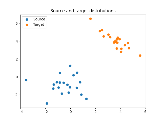
Generate data

n = 20  # nb samples

mu_s = np.array([-1, -1])
cov_s = np.array([[1, 0], [0, 1]])

mu_t = np.array([4, 4])
cov_t = np.array([[1, -0.8], [-0.8, 1]])

np.random.seed(0)
xs = ot.datasets.make_2D_samples_gauss(n, mu_s, cov_s)
xt = ot.datasets.make_2D_samples_gauss(n, mu_t, cov_t)

a, b = np.ones((n,)) / n, np.ones((n,)) / n  # uniform distribution on samples

# loss matrix
M = ot.dist(xs, xt)
M /= M.max()

Plot data

pl.figure(1)
pl.scatter(xs[:, 0], xs[:, 1], c="C0", label="Source")
pl.scatter(xt[:, 0], xt[:, 1], c="C1", label="Target")
pl.legend(loc=2)
pl.title("Source and target distributions")
pl.show()

Compute semi-relaxed and fully relaxed regularization paths

final_gamma = 1e-6
t, t_list, g_list = ot.regpath.regularization_path(
    a, b, M, reg=final_gamma, semi_relaxed=False
)
t2, t_list2, g_list2 = ot.regpath.regularization_path(
    a, b, M, reg=final_gamma, semi_relaxed=True
)

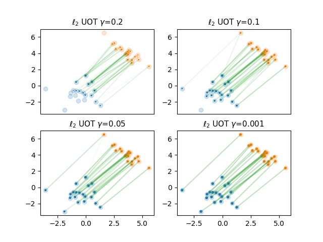
Plot the regularization path

The OT plan is plotted as a function of $gamma$ that is the inverse of the weight on the marginal relaxations.

pl.figure(2)
selected_gamma = [2e-1, 1e-1, 5e-2, 1e-3]
for p in range(4):
    tp = ot.regpath.compute_transport_plan(selected_gamma[p], g_list, t_list)
    P = tp.reshape((n, n))
    pl.subplot(2, 2, p + 1)
    if P.sum() > 0:
        P = P / P.max()
    for i in range(n):
        for j in range(n):
            if P[i, j] > 0:
                pl.plot(
                    [xs[i, 0], xt[j, 0]],
                    [xs[i, 1], xt[j, 1]],
                    color="C2",
                    alpha=P[i, j] * 0.3,
                )
    pl.scatter(xs[:, 0], xs[:, 1], c="C0", alpha=0.2)
    pl.scatter(xt[:, 0], xt[:, 1], c="C1", alpha=0.2)
    pl.scatter(
        xs[:, 0],
        xs[:, 1],
        c="C0",
        s=P.sum(1).ravel() * (1 + p) * 2,
        label="Re-weighted source",
        alpha=1,
    )
    pl.scatter(
        xt[:, 0],
        xt[:, 1],
        c="C1",
        s=P.sum(0).ravel() * (1 + p) * 2,
        label="Re-weighted target",
        alpha=1,
    )
    pl.plot([], [], color="C2", alpha=0.8, label="OT plan")
    pl.title(r"$\ell_2$ UOT $\gamma$={}".format(selected_gamma[p]), fontsize=11)
    if p < 2:
        pl.xticks(())
pl.show()

Animation of the regpath for UOT l2

nv = 50
g_list_v = np.logspace(-0.5, -2.5, nv)

pl.figure(3)


def _update_plot(iv):
    pl.clf()
    tp = ot.regpath.compute_transport_plan(g_list_v[iv], g_list, t_list)
    P = tp.reshape((n, n))
    if P.sum() > 0:
        P = P / P.max()
    for i in range(n):
        for j in range(n):
            if P[i, j] > 0:
                pl.plot(
                    [xs[i, 0], xt[j, 0]],
                    [xs[i, 1], xt[j, 1]],
                    color="C2",
                    alpha=P[i, j] * 0.5,
                )
    pl.scatter(xs[:, 0], xs[:, 1], c="C0", alpha=0.2)
    pl.scatter(xt[:, 0], xt[:, 1], c="C1", alpha=0.2)
    pl.scatter(
        xs[:, 0],
        xs[:, 1],
        c="C0",
        s=P.sum(1).ravel() * (1 + p) * 4,
        label="Re-weighted source",
        alpha=1,
    )
    pl.scatter(
        xt[:, 0],
        xt[:, 1],
        c="C1",
        s=P.sum(0).ravel() * (1 + p) * 4,
        label="Re-weighted target",
        alpha=1,
    )
    pl.plot([], [], color="C2", alpha=0.8, label="OT plan")
    pl.title(r"$\ell_2$ UOT $\gamma$={:1.3f}".format(g_list_v[iv]), fontsize=11)
    return 1


i = 0
_update_plot(i)

ani = animation.FuncAnimation(
    pl.gcf(), _update_plot, nv, interval=100, repeat_delay=2000
)

Once Loop Reflect

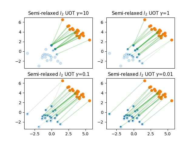
Plot the semi-relaxed regularization path

pl.figure(4)
selected_gamma = [10, 1, 1e-1, 1e-2]
for p in range(4):
    tp = ot.regpath.compute_transport_plan(selected_gamma[p], g_list2, t_list2)
    P = tp.reshape((n, n))
    pl.subplot(2, 2, p + 1)
    if P.sum() > 0:
        P = P / P.max()
    for i in range(n):
        for j in range(n):
            if P[i, j] > 0:
                pl.plot(
                    [xs[i, 0], xt[j, 0]],
                    [xs[i, 1], xt[j, 1]],
                    color="C2",
                    alpha=P[i, j] * 0.3,
                )
    pl.scatter(xs[:, 0], xs[:, 1], c="C0", alpha=0.2)
    pl.scatter(xt[:, 0], xt[:, 1], c="C1", alpha=1, label="Target marginal")
    pl.scatter(
        xs[:, 0],
        xs[:, 1],
        c="C0",
        s=P.sum(1).ravel() * 2 * (1 + p),
        label="Source marginal",
        alpha=1,
    )
    pl.plot([], [], color="C2", alpha=0.8, label="OT plan")
    pl.title(
        r"Semi-relaxed $l_2$ UOT $\gamma$={}".format(selected_gamma[p]), fontsize=11
    )
    if p < 2:
        pl.xticks(())
pl.show()

Animation of the regpath for semi-relaxed UOT l2

nv = 50
g_list_v = np.logspace(2, -2, nv)

pl.figure(5)


def _update_plot(iv):
    pl.clf()
    tp = ot.regpath.compute_transport_plan(g_list_v[iv], g_list2, t_list2)
    P = tp.reshape((n, n))
    if P.sum() > 0:
        P = P / P.max()
    for i in range(n):
        for j in range(n):
            if P[i, j] > 0:
                pl.plot(
                    [xs[i, 0], xt[j, 0]],
                    [xs[i, 1], xt[j, 1]],
                    color="C2",
                    alpha=P[i, j] * 0.5,
                )
    pl.scatter(xs[:, 0], xs[:, 1], c="C0", alpha=0.2)
    pl.scatter(xt[:, 0], xt[:, 1], c="C1", alpha=0.2)
    pl.scatter(
        xs[:, 0],
        xs[:, 1],
        c="C0",
        s=P.sum(1).ravel() * (1 + p) * 4,
        label="Re-weighted source",
        alpha=1,
    )
    pl.scatter(
        xt[:, 0],
        xt[:, 1],
        c="C1",
        s=P.sum(0).ravel() * (1 + p) * 4,
        label="Re-weighted target",
        alpha=1,
    )
    pl.plot([], [], color="C2", alpha=0.8, label="OT plan")
    pl.title(
        r"Semi-relaxed $\ell_2$ UOT $\gamma$={:1.3f}".format(g_list_v[iv]), fontsize=11
    )
    return 1


i = 0
_update_plot(i)

ani = animation.FuncAnimation(
    pl.gcf(), _update_plot, nv, interval=100, repeat_delay=2000
)

Once Loop Reflect