Row and column alignments with CO-Optimal Transport

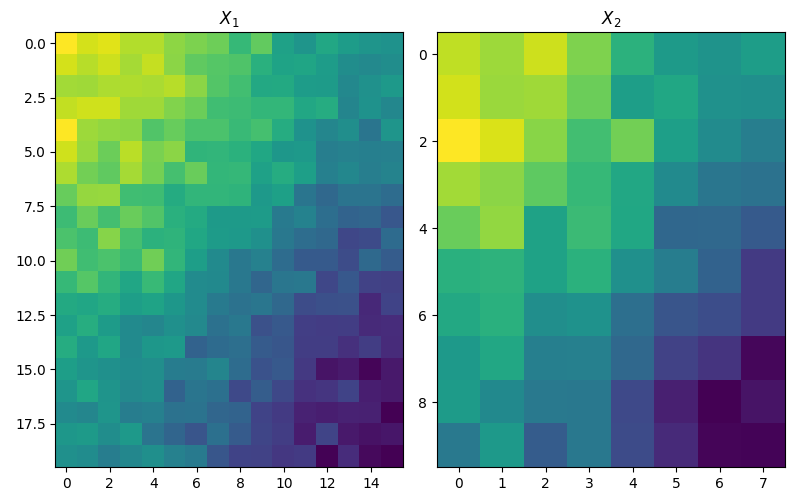
This example is designed to show how to use the CO-Optimal Transport [47]_ in POT. CO-Optimal Transport allows to calculate the distance between two arbitrary-size matrices, and to align their rows and columns. In this example, we consider two random matrices \(X_1\) and \(X_2\) defined by \((X_1)_{i,j} = \cos(\frac{i}{n_1} \pi) + \cos(\frac{j}{d_1} \pi) + \sigma \mathcal N(0,1)\) and \((X_2)_{i,j} = \cos(\frac{i}{n_2} \pi) + \cos(\frac{j}{d_2} \pi) + \sigma \mathcal N(0,1)\).

[49]

Redko, I., Vayer, T., Flamary, R., and Courty, N. (2020). CO-Optimal Transport. Advances in Neural Information Processing Systems, 33.

# Author: Remi Flamary <remi.flamary@unice.fr>
#         Quang Huy Tran <quang-huy.tran@univ-ubs.fr>
# License: MIT License

from matplotlib.patches import ConnectionPatch
import matplotlib.pylab as pl
import numpy as np
from ot.coot import co_optimal_transport as coot
from ot.coot import co_optimal_transport2 as coot2

Generating two random matrices

n1 = 20
n2 = 10
d1 = 16
d2 = 8
sigma = 0.2

X1 = (
    np.cos(np.arange(n1) * np.pi / n1)[:, None] +
    np.cos(np.arange(d1) * np.pi / d1)[None, :] +
    sigma * np.random.randn(n1, d1)
)
X2 = (
    np.cos(np.arange(n2) * np.pi / n2)[:, None] +
    np.cos(np.arange(d2) * np.pi / d2)[None, :] +
    sigma * np.random.randn(n2, d2)
)

Visualizing the matrices

pl.figure(1, (8, 5))
pl.subplot(1, 2, 1)
pl.imshow(X1)
pl.title('$X_1$')

pl.subplot(1, 2, 2)
pl.imshow(X2)
pl.title("$X_2$")

pl.tight_layout()

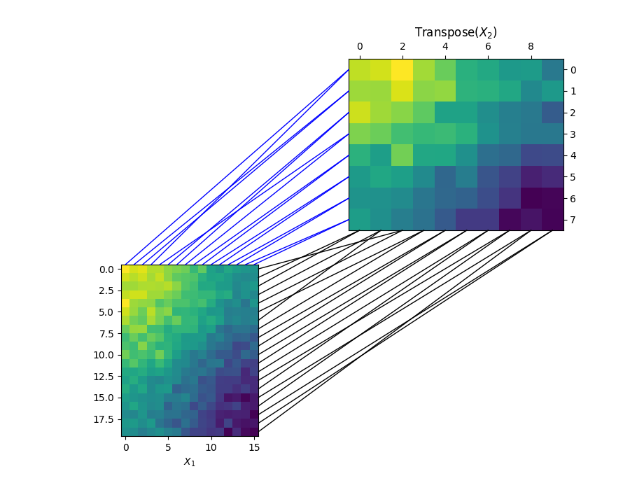
Visualizing the alignments of rows and columns, and calculating the CO-Optimal Transport distance

pi_sample, pi_feature, log = coot(X1, X2, log=True, verbose=True)
coot_distance = coot2(X1, X2)
print('CO-Optimal Transport distance = {:.5f}'.format(coot_distance))

fig = pl.figure(4, (9, 7))
pl.clf()

ax1 = pl.subplot(2, 2, 3)
pl.imshow(X1)
pl.xlabel('$X_1$')

ax2 = pl.subplot(2, 2, 2)
ax2.yaxis.tick_right()
pl.imshow(np.transpose(X2))
pl.title("Transpose($X_2$)")
ax2.xaxis.tick_top()

for i in range(n1):
    j = np.argmax(pi_sample[i, :])
    xyA = (d1 - .5, i)
    xyB = (j, d2 - .5)
    con = ConnectionPatch(xyA=xyA, xyB=xyB, coordsA=ax1.transData,
                          coordsB=ax2.transData, color="black")
    fig.add_artist(con)

for i in range(d1):
    j = np.argmax(pi_feature[i, :])
    xyA = (i, -.5)
    xyB = (-.5, j)
    con = ConnectionPatch(
        xyA=xyA, xyB=xyB, coordsA=ax1.transData, coordsB=ax2.transData, color="blue")
    fig.add_artist(con)

CO-Optimal Transport cost at iteration 1: 0.10903416567681642
CO-Optimal Transport cost at iteration 2: 0.0987568083692249
CO-Optimal Transport cost at iteration 3: 0.09685398028260428
CO-Optimal Transport distance = 0.09685