Partial Wasserstein and Gromov-Wasserstein example

This example is designed to show how to use the Partial (Gromov-)Wassertsein distance computation in POT.

# Author: Laetitia Chapel <laetitia.chapel@irisa.fr>
# License: MIT License

# necessary for 3d plot even if not used
from mpl_toolkits.mplot3d import Axes3D  # noqa
import scipy as sp
import numpy as np
import matplotlib.pylab as pl
import ot

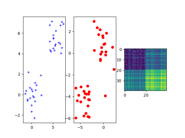
Sample two 2D Gaussian distributions and plot them

For demonstration purpose, we sample two Gaussian distributions in 2-d spaces and add some random noise.

n_samples = 20  # nb samples (gaussian)
n_noise = 20  # nb of samples (noise)

mu = np.array([0, 0])
cov = np.array([[1, 0], [0, 2]])

xs = ot.datasets.make_2D_samples_gauss(n_samples, mu, cov)
xs = np.append(xs, (np.random.rand(n_noise, 2) + 1) * 4).reshape((-1, 2))
xt = ot.datasets.make_2D_samples_gauss(n_samples, mu, cov)
xt = np.append(xt, (np.random.rand(n_noise, 2) + 1) * -3).reshape((-1, 2))

M = sp.spatial.distance.cdist(xs, xt)

fig = pl.figure()
ax1 = fig.add_subplot(131)
ax1.plot(xs[:, 0], xs[:, 1], '+b', label='Source samples')
ax2 = fig.add_subplot(132)
ax2.scatter(xt[:, 0], xt[:, 1], color='r')
ax3 = fig.add_subplot(133)
ax3.imshow(M)
pl.show()

Out:

/home/circleci/project/examples/plot_partial_wass_and_gromov.py:51: UserWarning: Matplotlib is currently using agg, which is a non-GUI backend, so cannot show the figure.
  pl.show()

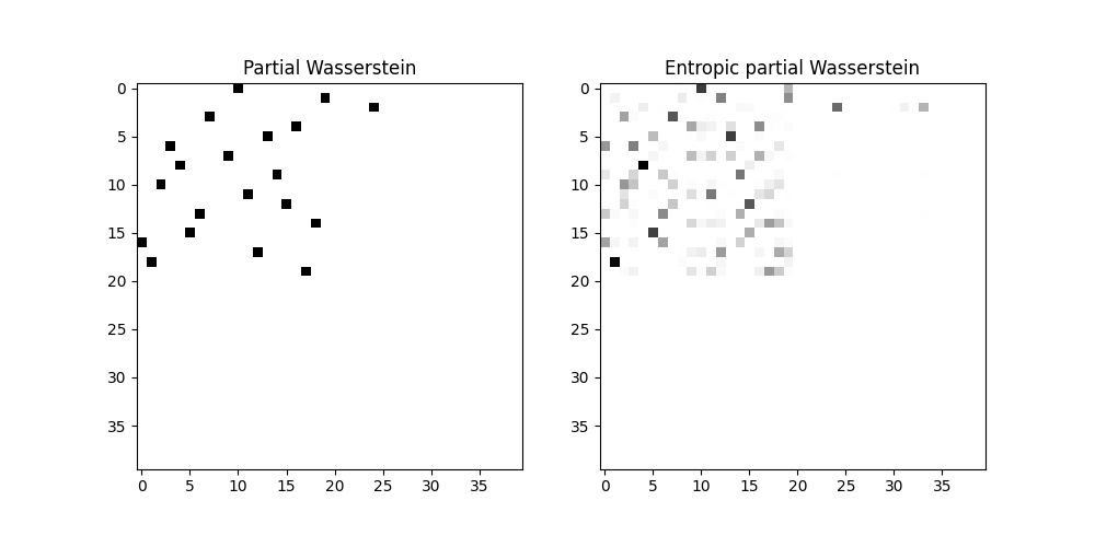
Compute partial Wasserstein plans and distance

p = ot.unif(n_samples + n_noise)
q = ot.unif(n_samples + n_noise)

w0, log0 = ot.partial.partial_wasserstein(p, q, M, m=0.5, log=True)
w, log = ot.partial.entropic_partial_wasserstein(p, q, M, reg=0.1, m=0.5,
                                                 log=True)

print('Partial Wasserstein distance (m = 0.5): ' + str(log0['partial_w_dist']))
print('Entropic partial Wasserstein distance (m = 0.5): ' +
      str(log['partial_w_dist']))

pl.figure(1, (10, 5))
pl.subplot(1, 2, 1)
pl.imshow(w0, cmap='jet')
pl.title('Partial Wasserstein')
pl.subplot(1, 2, 2)
pl.imshow(w, cmap='jet')
pl.title('Entropic partial Wasserstein')
pl.show()

Out:

Partial Wasserstein distance (m = 0.5): 0.5049910717015967
Entropic partial Wasserstein distance (m = 0.5): 0.5228286857800669
/home/circleci/project/examples/plot_partial_wass_and_gromov.py:76: UserWarning: Matplotlib is currently using agg, which is a non-GUI backend, so cannot show the figure.
  pl.show()

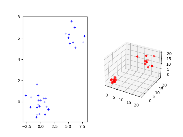
Sample one 2D and 3D Gaussian distributions and plot them

The Gromov-Wasserstein distance allows to compute distances with samples that do not belong to the same metric space. For demonstration purpose, we sample two Gaussian distributions in 2- and 3-dimensional spaces.

n_samples = 20  # nb samples
n_noise = 10  # nb of samples (noise)

p = ot.unif(n_samples + n_noise)
q = ot.unif(n_samples + n_noise)

mu_s = np.array([0, 0])
cov_s = np.array([[1, 0], [0, 1]])

mu_t = np.array([0, 0, 0])
cov_t = np.array([[1, 0, 0], [0, 1, 0], [0, 0, 1]])


xs = ot.datasets.make_2D_samples_gauss(n_samples, mu_s, cov_s)
xs = np.concatenate((xs, ((np.random.rand(n_noise, 2) + 1) * 4)), axis=0)
P = sp.linalg.sqrtm(cov_t)
xt = np.random.randn(n_samples, 3).dot(P) + mu_t
xt = np.concatenate((xt, ((np.random.rand(n_noise, 3) + 1) * 10)), axis=0)

fig = pl.figure()
ax1 = fig.add_subplot(121)
ax1.plot(xs[:, 0], xs[:, 1], '+b', label='Source samples')
ax2 = fig.add_subplot(122, projection='3d')
ax2.scatter(xt[:, 0], xt[:, 1], xt[:, 2], color='r')
pl.show()

Out:

/home/circleci/project/examples/plot_partial_wass_and_gromov.py:112: UserWarning: Matplotlib is currently using agg, which is a non-GUI backend, so cannot show the figure.
  pl.show()

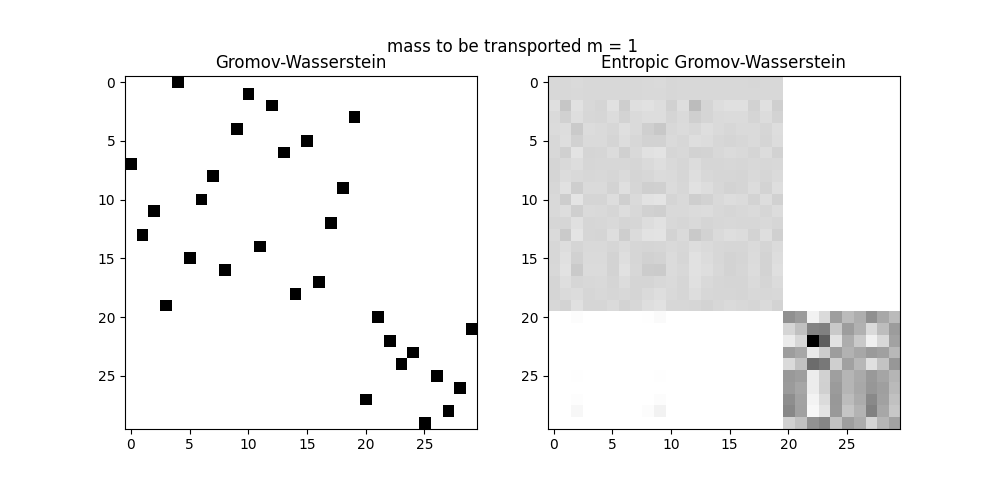
Compute partial Gromov-Wasserstein plans and distance

C1 = sp.spatial.distance.cdist(xs, xs)
C2 = sp.spatial.distance.cdist(xt, xt)

# transport 100% of the mass
print('-----m = 1')
m = 1
res0, log0 = ot.partial.partial_gromov_wasserstein(C1, C2, p, q, m=m, log=True)
res, log = ot.partial.entropic_partial_gromov_wasserstein(C1, C2, p, q, 10,
                                                          m=m, log=True)

print('Wasserstein distance (m = 1): ' + str(log0['partial_gw_dist']))
print('Entropic Wasserstein distance (m = 1): ' + str(log['partial_gw_dist']))

pl.figure(1, (10, 5))
pl.title("mass to be transported m = 1")
pl.subplot(1, 2, 1)
pl.imshow(res0, cmap='jet')
pl.title('Wasserstein')
pl.subplot(1, 2, 2)
pl.imshow(res, cmap='jet')
pl.title('Entropic Wasserstein')
pl.show()

# transport 2/3 of the mass
print('-----m = 2/3')
m = 2 / 3
res0, log0 = ot.partial.partial_gromov_wasserstein(C1, C2, p, q, m=m, log=True)
res, log = ot.partial.entropic_partial_gromov_wasserstein(C1, C2, p, q, 10,
                                                          m=m, log=True)

print('Partial Wasserstein distance (m = 2/3): ' +
      str(log0['partial_gw_dist']))
print('Entropic partial Wasserstein distance (m = 2/3): ' +
      str(log['partial_gw_dist']))

pl.figure(1, (10, 5))
pl.title("mass to be transported m = 2/3")
pl.subplot(1, 2, 1)
pl.imshow(res0, cmap='jet')
pl.title('Partial Wasserstein')
pl.subplot(1, 2, 2)
pl.imshow(res, cmap='jet')
pl.title('Entropic partial Wasserstein')
pl.show()

Out:

-----m = 1
Wasserstein distance (m = 1): 75.79016141286937
Entropic Wasserstein distance (m = 1): 76.89766951491862
/home/circleci/project/examples/plot_partial_wass_and_gromov.py:141: UserWarning: Matplotlib is currently using agg, which is a non-GUI backend, so cannot show the figure.
  pl.show()
-----m = 2/3
Partial Wasserstein distance (m = 2/3): 0.17256960007764344
Entropic partial Wasserstein distance (m = 2/3): 1.0889592327112803
/home/circleci/project/examples/plot_partial_wass_and_gromov.py:157: MatplotlibDeprecationWarning: Adding an axes using the same arguments as a previous axes currently reuses the earlier instance.  In a future version, a new instance will always be created and returned.  Meanwhile, this warning can be suppressed, and the future behavior ensured, by passing a unique label to each axes instance.
  pl.subplot(1, 2, 1)
/home/circleci/project/examples/plot_partial_wass_and_gromov.py:160: MatplotlibDeprecationWarning: Adding an axes using the same arguments as a previous axes currently reuses the earlier instance.  In a future version, a new instance will always be created and returned.  Meanwhile, this warning can be suppressed, and the future behavior ensured, by passing a unique label to each axes instance.
  pl.subplot(1, 2, 2)
/home/circleci/project/examples/plot_partial_wass_and_gromov.py:163: UserWarning: Matplotlib is currently using agg, which is a non-GUI backend, so cannot show the figure.
  pl.show()