Wasserstein Discriminant Analysis

This example illustrate the use of WDA as proposed in [11].

[11] Flamary, R., Cuturi, M., Courty, N., & Rakotomamonjy, A. (2016). Wasserstein Discriminant Analysis.

# Author: Remi Flamary <remi.flamary@unice.fr>
#
# License: MIT License

import numpy as np
import matplotlib.pylab as pl

from ot.dr import wda, fda

Generate data

n = 1000  # nb samples in source and target datasets
nz = 0.2

# generate circle dataset
t = np.random.rand(n) * 2 * np.pi
ys = np.floor((np.arange(n) * 1.0 / n * 3)) + 1
xs = np.concatenate(
    (np.cos(t).reshape((-1, 1)), np.sin(t).reshape((-1, 1))), 1)
xs = xs * ys.reshape(-1, 1) + nz * np.random.randn(n, 2)

t = np.random.rand(n) * 2 * np.pi
yt = np.floor((np.arange(n) * 1.0 / n * 3)) + 1
xt = np.concatenate(
    (np.cos(t).reshape((-1, 1)), np.sin(t).reshape((-1, 1))), 1)
xt = xt * yt.reshape(-1, 1) + nz * np.random.randn(n, 2)

nbnoise = 8

xs = np.hstack((xs, np.random.randn(n, nbnoise)))
xt = np.hstack((xt, np.random.randn(n, nbnoise)))

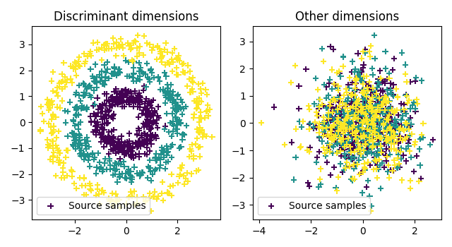
Plot data

pl.figure(1, figsize=(6.4, 3.5))

pl.subplot(1, 2, 1)
pl.scatter(xt[:, 0], xt[:, 1], c=ys, marker='+', label='Source samples')
pl.legend(loc=0)
pl.title('Discriminant dimensions')

pl.subplot(1, 2, 2)
pl.scatter(xt[:, 2], xt[:, 3], c=ys, marker='+', label='Source samples')
pl.legend(loc=0)
pl.title('Other dimensions')
pl.tight_layout()

Compute Fisher Discriminant Analysis

p = 2

Pfda, projfda = fda(xs, ys, p)

Compute Wasserstein Discriminant Analysis

p = 2
reg = 1e0
k = 10
maxiter = 100

Pwda, projwda = wda(xs, ys, p, reg, k, maxiter=maxiter)

Out:

Compiling cost function...
Computing gradient of cost function...
 iter              cost val         grad. norm
    1   +9.0425335111320371e-01 3.36728904e-01
    2   +5.0981248231952336e-01 3.49447291e-01
    3   +3.8456893521828645e-01 2.68836146e-01
    4   +3.1869445832391702e-01 2.50634853e-01
    5   +2.3255923811662640e-01 1.30829408e-01
    6   +2.2374089978244924e-01 8.22152912e-02
    7   +2.2197270706738836e-01 6.83068347e-02
    8   +2.1878886804008973e-01 8.41570320e-03
    9   +2.1874184588953391e-01 6.87975679e-04
   10   +2.1874152322647425e-01 1.25011225e-04
   11   +2.1874152180173498e-01 1.18603421e-04
   12   +2.1874151699082819e-01 8.16555830e-05
   13   +2.1874151270014219e-01 9.83233613e-06
   14   +2.1874151263659172e-01 1.00731914e-06
   15   +2.1874151263589317e-01 3.88549586e-07
Terminated - min grad norm reached after 15 iterations, 4.05 seconds.

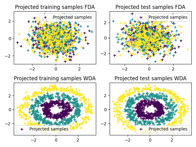
Plot 2D projections

xsp = projfda(xs)
xtp = projfda(xt)

xspw = projwda(xs)
xtpw = projwda(xt)

pl.figure(2)

pl.subplot(2, 2, 1)
pl.scatter(xsp[:, 0], xsp[:, 1], c=ys, marker='+', label='Projected samples')
pl.legend(loc=0)
pl.title('Projected training samples FDA')

pl.subplot(2, 2, 2)
pl.scatter(xtp[:, 0], xtp[:, 1], c=ys, marker='+', label='Projected samples')
pl.legend(loc=0)
pl.title('Projected test samples FDA')

pl.subplot(2, 2, 3)
pl.scatter(xspw[:, 0], xspw[:, 1], c=ys, marker='+', label='Projected samples')
pl.legend(loc=0)
pl.title('Projected training samples WDA')

pl.subplot(2, 2, 4)
pl.scatter(xtpw[:, 0], xtpw[:, 1], c=ys, marker='+', label='Projected samples')
pl.legend(loc=0)
pl.title('Projected test samples WDA')
pl.tight_layout()

pl.show()

Out:

/home/circleci/project/examples/plot_WDA.py:127: UserWarning: Matplotlib is currently using agg, which is a non-GUI backend, so cannot show the figure.
  pl.show()