Note
Click here to download the full example code
1D Wasserstein barycenter comparison between exact LP and entropic regularization
This example illustrates the computation of regularized Wasserstein Barycenter as proposed in [3] and exact LP barycenters using standard LP solver.
It reproduces approximately Figure 3.1 and 3.2 from the following paper: Cuturi, M., & Peyré, G. (2016). A smoothed dual approach for variational Wasserstein problems. SIAM Journal on Imaging Sciences, 9(1), 320-343.
[3] Benamou, J. D., Carlier, G., Cuturi, M., Nenna, L., & Peyré, G. (2015). Iterative Bregman projections for regularized transportation problems SIAM Journal on Scientific Computing, 37(2), A1111-A1138.
# Author: Remi Flamary <remi.flamary@unice.fr>
#
# License: MIT License

import numpy as np
import matplotlib.pylab as pl
import ot
# necessary for 3d plot even if not used
from mpl_toolkits.mplot3d import Axes3D  # noqa
from matplotlib.collections import PolyCollection  # noqa

#import ot.lp.cvx as cvx
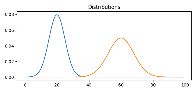
Gaussian Data
problems = []

n = 100  # nb bins

# bin positions
x = np.arange(n, dtype=np.float64)

# Gaussian distributions
# Gaussian distributions
a1 = ot.datasets.make_1D_gauss(n, m=20, s=5)  # m= mean, s= std
a2 = ot.datasets.make_1D_gauss(n, m=60, s=8)

# creating matrix A containing all distributions
A = np.vstack((a1, a2)).T
n_distributions = A.shape[1]

# loss matrix + normalization
M = ot.utils.dist0(n)
M /= M.max()
pl.figure(1, figsize=(6.4, 3))
for i in range(n_distributions):
    pl.plot(x, A[:, i])
pl.title('Distributions')
pl.tight_layout()
alpha = 0.5 # 0<=alpha<=1
weights = np.array([1 - alpha, alpha])
# l2bary
bary_l2 = A.dot(weights)
# wasserstein
reg = 1e-3
ot.tic()
bary_wass = ot.bregman.barycenter(A, M, reg, weights)
ot.toc()
ot.tic()
bary_wass2 = ot.lp.barycenter(A, M, weights, solver='interior-point', verbose=True)
ot.toc()
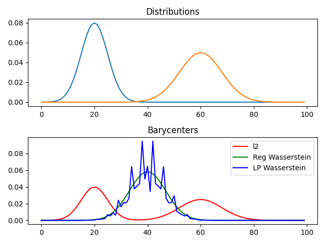
pl.figure(2)
pl.clf()
pl.subplot(2, 1, 1)
for i in range(n_distributions):
pl.plot(x, A[:, i])
pl.title('Distributions')
pl.subplot(2, 1, 2)
pl.plot(x, bary_l2, 'r', label='l2')
pl.plot(x, bary_wass, 'g', label='Reg Wasserstein')
pl.plot(x, bary_wass2, 'b', label='LP Wasserstein')
pl.legend()
pl.title('Barycenters')
pl.tight_layout()
problems.append([A, [bary_l2, bary_wass, bary_wass2]])
Out:
Elapsed time : 0.004806041717529297 s
Primal Feasibility  Dual Feasibility    Duality Gap         Step             Path Parameter      Objective
1.0                 1.0                 1.0                 -                1.0                 1700.336700337
0.006776453137633   0.006776453137633   0.006776453137633   0.9932238647293  0.006776453137633   125.6700527543
0.004018712867872   0.004018712867872   0.004018712867872   0.4301142633003  0.004018712867872   12.26594150092
0.001172775061628   0.001172775061628   0.001172775061628   0.7599932455024  0.001172775061628   0.3378536968899
0.0004375137005389  0.0004375137005389  0.0004375137005389  0.642233180799   0.0004375137005389  0.1468420566359
0.0002326690467335  0.0002326690467335  0.0002326690467335  0.5016999460911  0.0002326690467335  0.09381703231417
7.430121674289e-05  7.430121674289e-05  7.430121674289e-05  0.7035962305811  7.430121674289e-05  0.05777870257166
5.321227839112e-05  5.321227839109e-05  5.321227839112e-05  0.3087841864049  5.321227839112e-05  0.05266249477258
1.990900379259e-05  1.990900379259e-05  1.990900379259e-05  0.6520472013337  1.990900379259e-05  0.04526054405532
6.305442046961e-06  6.305442046986e-06  6.305442046961e-06  0.7073953304095  6.305442046961e-06  0.04237597591386
2.290148391626e-06  2.290148391615e-06  2.290148391629e-06  0.6941812711509  2.290148391642e-06  0.04152284932101
1.182864875683e-06  1.182864875753e-06  1.18286487577e-06   0.50845520453    1.182864875789e-06  0.04129461872834
3.626786383939e-07  3.626786384381e-07  3.626786384359e-07  0.7101651571784  3.626786383978e-07  0.04113032448925
1.539754244823e-07  1.539754251533e-07  1.53975425164e-07   0.62793220614    1.539754255888e-07  0.04108867636383
5.19322169473e-08   5.193221785387e-08  5.19322178167e-08   0.6843453235232  5.193221967538e-08  0.04106859618467
1.888204871963e-08  1.888204395725e-08  1.888204397257e-08  0.6673445060343  1.888205318427e-08  0.04106214175139
5.676863452177e-09  5.676860441977e-09  5.676860407912e-09  0.728170207609   5.676889409915e-09  0.04105958648799
3.501141895059e-09  3.501129003556e-09  3.501129013359e-09  0.4140256354197  3.50114157346e-09   0.04105916264834
1.110588836154e-09  1.110579164619e-09  1.110579244827e-09  0.6998966971497  1.110627540446e-09  0.04105870073351
5.771256718227e-10  5.772171357666e-10  5.772172245844e-10  0.4999961139223  5.770013760958e-10  0.04105859769037
1.534527723964e-10  1.536571417282e-10  1.536571732899e-10  0.7517045323913  1.535845988547e-10  0.04105851679395
6.720074578141e-11  6.738590511283e-11  6.738598807526e-11  0.5944088032552  6.735313147595e-11  0.04105850033861
1.767193623342e-11  1.746713504798e-11  1.746721851974e-11  0.7557993816051  1.741701168899e-11  0.04105849090432
Optimization terminated successfully.
         Current function value: 0.041058
         Iterations: 22
Elapsed time : 2.2309346199035645 s
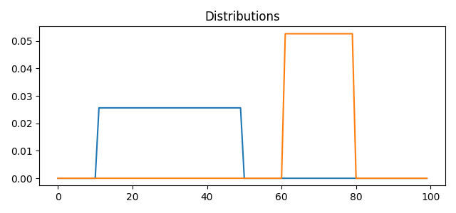
Stair Data
pl.figure(1, figsize=(6.4, 3))
for i in range(n_distributions):
    pl.plot(x, A[:, i])
pl.title('Distributions')
pl.tight_layout()
alpha = 0.5 # 0<=alpha<=1
weights = np.array([1 - alpha, alpha])
# l2bary
bary_l2 = A.dot(weights)
# wasserstein
reg = 1e-3
ot.tic()
bary_wass = ot.bregman.barycenter(A, M, reg, weights)
ot.toc()
ot.tic()
bary_wass2 = ot.lp.barycenter(A, M, weights, solver='interior-point', verbose=True)
ot.toc()
problems.append([A, [bary_l2, bary_wass, bary_wass2]])
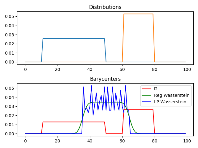
pl.figure(2)
pl.clf()
pl.subplot(2, 1, 1)
for i in range(n_distributions):
pl.plot(x, A[:, i])
pl.title('Distributions')
pl.subplot(2, 1, 2)
pl.plot(x, bary_l2, 'r', label='l2')
pl.plot(x, bary_wass, 'g', label='Reg Wasserstein')
pl.plot(x, bary_wass2, 'b', label='LP Wasserstein')
pl.legend()
pl.title('Barycenters')
pl.tight_layout()
Out:
Elapsed time : 0.006773233413696289 s
Primal Feasibility  Dual Feasibility    Duality Gap         Step             Path Parameter      Objective
1.0                 1.0                 1.0                 -                1.0                 1700.336700337
0.006776466288964   0.006776466288964   0.006776466288964   0.9932238515788  0.006776466288964   125.6649255807
0.004036918865493   0.004036918865493   0.004036918865493   0.4272973099317  0.004036918865493   12.34716170109
0.00121923268707    0.00121923268707    0.00121923268707    0.7496986855987  0.00121923268707    0.3243835647409
0.0003837422984435  0.0003837422984435  0.0003837422984435  0.6926882608283  0.0003837422984435  0.1361719397493
0.0001070128410184  0.0001070128410185  0.0001070128410184  0.7643889137854  0.0001070128410184  0.0758195283252
0.0001001275033712  0.0001001275033712  0.0001001275033712  0.07058704837825 0.0001001275033712  0.07347394936351
4.550897507858e-05  4.550897507855e-05  4.550897507858e-05  0.5761172484818  4.550897507858e-05  0.05555077655051
8.557124125543e-06  8.55712412556e-06   8.557124125544e-06  0.8535925441153  8.557124125544e-06  0.04439814660222
3.611995628439e-06  3.611995628483e-06  3.611995628447e-06  0.6002277331523  3.611995628448e-06  0.04283007762153
7.59039375036e-07   7.590393750537e-07  7.590393750377e-07  0.8221486533444  7.590393750377e-07  0.04192322976248
8.299929287393e-08  8.299929290147e-08  8.299929287538e-08  0.90174679388    8.299929287582e-08  0.04170825633295
3.11756020056e-10   3.117560224267e-10  3.117560198724e-10  0.9970399692265  3.117560198862e-10  0.04168179329766
1.559765619625e-14  1.562166058542e-14  1.559756940692e-14  0.9999499686772  1.559749451091e-14  0.04168169240444
Optimization terminated successfully.
         Current function value: 0.041682
         Iterations: 13
Elapsed time : 2.114680051803589 s
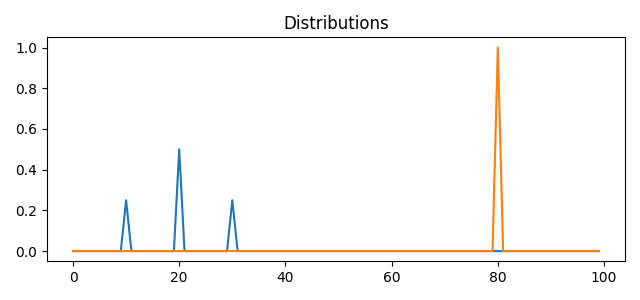
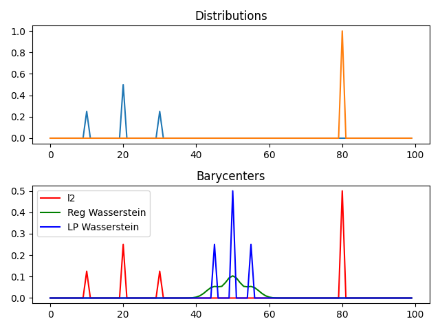
Dirac Data
pl.figure(1, figsize=(6.4, 3))
for i in range(n_distributions):
    pl.plot(x, A[:, i])
pl.title('Distributions')
pl.tight_layout()
alpha = 0.5  # 0<=alpha<=1
weights = np.array([1 - alpha, alpha])

# l2bary
bary_l2 = A.dot(weights)

# wasserstein
reg = 1e-3
ot.tic()
bary_wass = ot.bregman.barycenter(A, M, reg, weights)
ot.toc()


ot.tic()
bary_wass2 = ot.lp.barycenter(A, M, weights, solver='interior-point', verbose=True)
ot.toc()


problems.append([A, [bary_l2, bary_wass, bary_wass2]])

pl.figure(2)
pl.clf()
pl.subplot(2, 1, 1)
for i in range(n_distributions):
    pl.plot(x, A[:, i])
pl.title('Distributions')

pl.subplot(2, 1, 2)
pl.plot(x, bary_l2, 'r', label='l2')
pl.plot(x, bary_wass, 'g', label='Reg Wasserstein')
pl.plot(x, bary_wass2, 'b', label='LP Wasserstein')
pl.legend()
pl.title('Barycenters')
pl.tight_layout()
Out:
Elapsed time : 0.0020160675048828125 s
Primal Feasibility  Dual Feasibility    Duality Gap         Step             Path Parameter      Objective
1.0                 1.0                 1.0                 -                1.0                 1700.336700337
0.006774675520725   0.006774675520725   0.006774675520725   0.9932256422636  0.006774675520725   125.6956034742
0.002048208707565   0.002048208707565   0.002048208707565   0.7343095368139  0.002048208707565   5.213991622129
0.0002697365474771  0.0002697365474771  0.0002697365474771  0.88394035012    0.0002697365474771  0.5059383903874
6.832109993947e-05  6.832109993948e-05  6.832109993947e-05  0.7601171075956  6.832109993947e-05  0.2339657807271
2.437682932215e-05  2.437682932216e-05  2.437682932215e-05  0.6663448297482  2.437682932215e-05  0.1471256246324
1.13498321631e-05   1.134983216308e-05  1.13498321631e-05   0.5553643816395  1.13498321631e-05   0.1181584941171
3.342312725893e-06  3.342312725884e-06  3.342312725893e-06  0.7238133571609  3.342312725893e-06  0.1006387519747
7.07856123164e-07   7.078561231657e-07  7.078561231639e-07  0.8033142552506  7.078561231639e-07  0.0947473464627
1.966870955747e-07  1.966870953549e-07  1.966870953535e-07  0.7525479179267  1.966870953847e-07  0.09354342735762
4.199895276708e-10  4.199895327841e-10  4.199895261516e-10  0.9984019849274  4.199895261919e-10  0.09310367785861
2.101147576949e-14  2.102008538586e-14  2.101155996689e-14  0.9999499712639  2.101155824779e-14  0.09310274466459
Optimization terminated successfully.
         Current function value: 0.093103
         Iterations: 11
Elapsed time : 2.7300755977630615 s
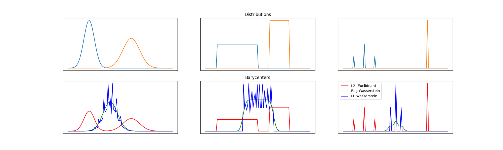
Final figure
nbm = len(problems)
nbm2 = (nbm // 2)


pl.figure(2, (20, 6))
pl.clf()

for i in range(nbm):

    A = problems[i][0]
    bary_l2 = problems[i][1][0]
    bary_wass = problems[i][1][1]
    bary_wass2 = problems[i][1][2]

    pl.subplot(2, nbm, 1 + i)
    for j in range(n_distributions):
        pl.plot(x, A[:, j])
    if i == nbm2:
        pl.title('Distributions')
    pl.xticks(())
    pl.yticks(())

    pl.subplot(2, nbm, 1 + i + nbm)

    pl.plot(x, bary_l2, 'r', label='L2 (Euclidean)')
    pl.plot(x, bary_wass, 'g', label='Reg Wasserstein')
    pl.plot(x, bary_wass2, 'b', label='LP Wasserstein')
    if i == nbm - 1:
        pl.legend()
    if i == nbm2:
        pl.title('Barycenters')

    pl.xticks(())
    pl.yticks(())
Total running time of the script: ( 0 minutes 8.217 seconds)