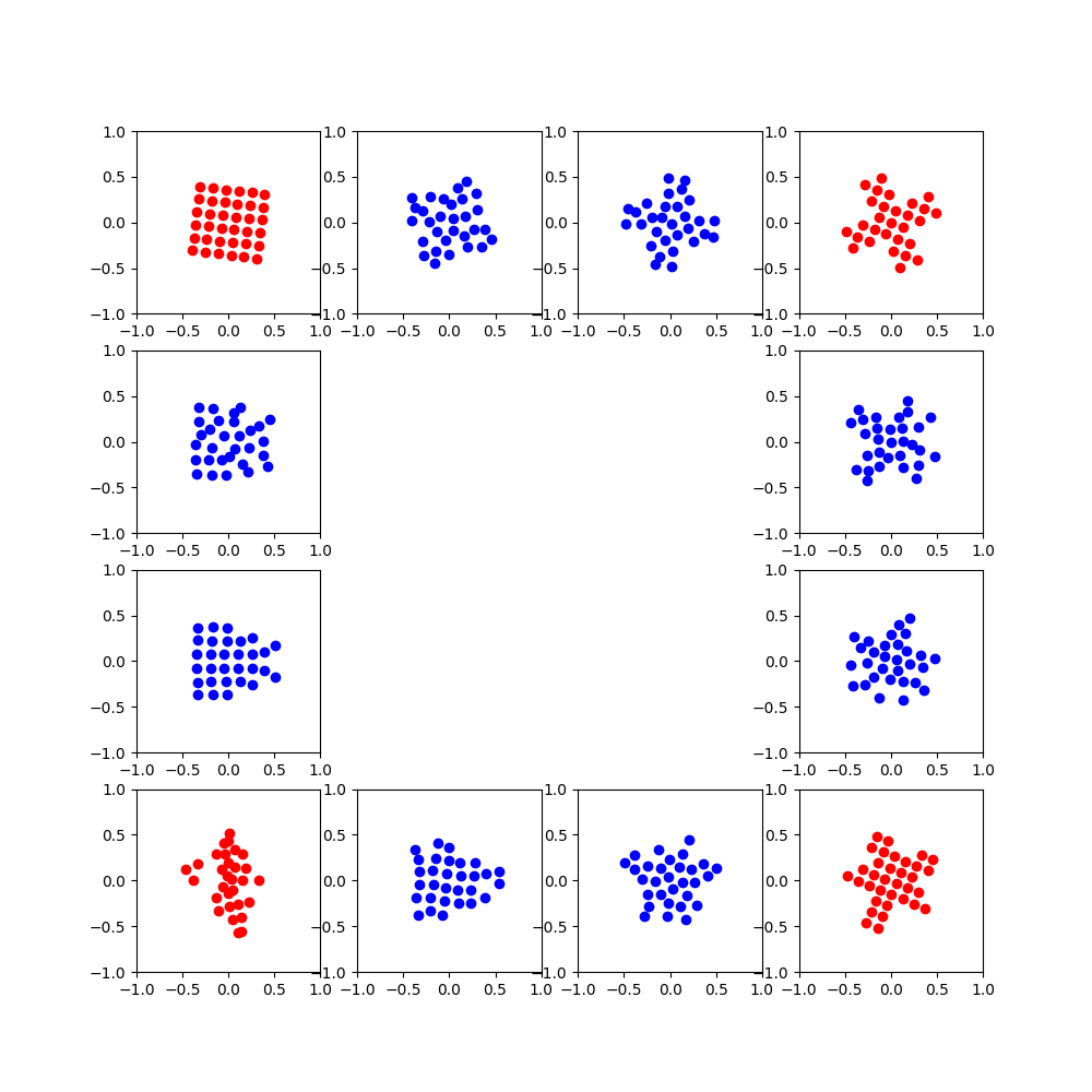
Gromov-Wasserstein Barycenter example

This example is designed to show how to use the Gromov-Wasserstein distance computation in POT.

# Author: Erwan Vautier <erwan.vautier@gmail.com>
#         Nicolas Courty <ncourty@irisa.fr>
#
# License: MIT License


import numpy as np
import scipy as sp

import matplotlib.pylab as pl
from sklearn import manifold
from sklearn.decomposition import PCA

import ot

Smacof MDS

This function allows to find an embedding of points given a dissimilarity matrix that will be given by the output of the algorithm

def smacof_mds(C, dim, max_iter=3000, eps=1e-9):
    """
    Returns an interpolated point cloud following the dissimilarity matrix C
    using SMACOF multidimensional scaling (MDS) in specific dimensionned
    target space

    Parameters
    ----------
    C : ndarray, shape (ns, ns)
        dissimilarity matrix
    dim : int
          dimension of the targeted space
    max_iter :  int
        Maximum number of iterations of the SMACOF algorithm for a single run
    eps : float
        relative tolerance w.r.t stress to declare converge

    Returns
    -------
    npos : ndarray, shape (R, dim)
           Embedded coordinates of the interpolated point cloud (defined with
           one isometry)
    """

    rng = np.random.RandomState(seed=3)

    mds = manifold.MDS(
        dim,
        max_iter=max_iter,
        eps=1e-9,
        dissimilarity='precomputed',
        n_init=1)
    pos = mds.fit(C).embedding_

    nmds = manifold.MDS(
        2,
        max_iter=max_iter,
        eps=1e-9,
        dissimilarity="precomputed",
        random_state=rng,
        n_init=1)
    npos = nmds.fit_transform(C, init=pos)

    return npos

Data preparation

The four distributions are constructed from 4 simple images

def im2mat(I):
    """Converts and image to matrix (one pixel per line)"""
    return I.reshape((I.shape[0] * I.shape[1], I.shape[2]))


square = pl.imread('../data/square.png').astype(np.float64)[:, :, 2]
cross = pl.imread('../data/cross.png').astype(np.float64)[:, :, 2]
triangle = pl.imread('../data/triangle.png').astype(np.float64)[:, :, 2]
star = pl.imread('../data/star.png').astype(np.float64)[:, :, 2]

shapes = [square, cross, triangle, star]

S = 4
xs = [[] for i in range(S)]


for nb in range(4):
    for i in range(8):
        for j in range(8):
            if shapes[nb][i, j] < 0.95:
                xs[nb].append([j, 8 - i])

xs = np.array([np.array(xs[0]), np.array(xs[1]),
               np.array(xs[2]), np.array(xs[3])])

Barycenter computation

ns = [len(xs[s]) for s in range(S)]
n_samples = 30

"""Compute all distances matrices for the four shapes"""
Cs = [sp.spatial.distance.cdist(xs[s], xs[s]) for s in range(S)]
Cs = [cs / cs.max() for cs in Cs]

ps = [ot.unif(ns[s]) for s in range(S)]
p = ot.unif(n_samples)


lambdast = [[float(i) / 3, float(3 - i) / 3] for i in [1, 2]]

Ct01 = [0 for i in range(2)]
for i in range(2):
    Ct01[i] = ot.gromov.gromov_barycenters(n_samples, [Cs[0], Cs[1]],
                                           [ps[0], ps[1]
                                            ], p, lambdast[i], 'square_loss',  # 5e-4,
                                           max_iter=100, tol=1e-3)

Ct02 = [0 for i in range(2)]
for i in range(2):
    Ct02[i] = ot.gromov.gromov_barycenters(n_samples, [Cs[0], Cs[2]],
                                           [ps[0], ps[2]
                                            ], p, lambdast[i], 'square_loss',  # 5e-4,
                                           max_iter=100, tol=1e-3)

Ct13 = [0 for i in range(2)]
for i in range(2):
    Ct13[i] = ot.gromov.gromov_barycenters(n_samples, [Cs[1], Cs[3]],
                                           [ps[1], ps[3]
                                            ], p, lambdast[i], 'square_loss',  # 5e-4,
                                           max_iter=100, tol=1e-3)

Ct23 = [0 for i in range(2)]
for i in range(2):
    Ct23[i] = ot.gromov.gromov_barycenters(n_samples, [Cs[2], Cs[3]],
                                           [ps[2], ps[3]
                                            ], p, lambdast[i], 'square_loss',  # 5e-4,
                                           max_iter=100, tol=1e-3)

Visualization

The PCA helps in getting consistency between the rotations

clf = PCA(n_components=2)
npos = [0, 0, 0, 0]
npos = [smacof_mds(Cs[s], 2) for s in range(S)]

npost01 = [0, 0]
npost01 = [smacof_mds(Ct01[s], 2) for s in range(2)]
npost01 = [clf.fit_transform(npost01[s]) for s in range(2)]

npost02 = [0, 0]
npost02 = [smacof_mds(Ct02[s], 2) for s in range(2)]
npost02 = [clf.fit_transform(npost02[s]) for s in range(2)]

npost13 = [0, 0]
npost13 = [smacof_mds(Ct13[s], 2) for s in range(2)]
npost13 = [clf.fit_transform(npost13[s]) for s in range(2)]

npost23 = [0, 0]
npost23 = [smacof_mds(Ct23[s], 2) for s in range(2)]
npost23 = [clf.fit_transform(npost23[s]) for s in range(2)]


fig = pl.figure(figsize=(10, 10))

ax1 = pl.subplot2grid((4, 4), (0, 0))
pl.xlim((-1, 1))
pl.ylim((-1, 1))
ax1.scatter(npos[0][:, 0], npos[0][:, 1], color='r')

ax2 = pl.subplot2grid((4, 4), (0, 1))
pl.xlim((-1, 1))
pl.ylim((-1, 1))
ax2.scatter(npost01[1][:, 0], npost01[1][:, 1], color='b')

ax3 = pl.subplot2grid((4, 4), (0, 2))
pl.xlim((-1, 1))
pl.ylim((-1, 1))
ax3.scatter(npost01[0][:, 0], npost01[0][:, 1], color='b')

ax4 = pl.subplot2grid((4, 4), (0, 3))
pl.xlim((-1, 1))
pl.ylim((-1, 1))
ax4.scatter(npos[1][:, 0], npos[1][:, 1], color='r')

ax5 = pl.subplot2grid((4, 4), (1, 0))
pl.xlim((-1, 1))
pl.ylim((-1, 1))
ax5.scatter(npost02[1][:, 0], npost02[1][:, 1], color='b')

ax6 = pl.subplot2grid((4, 4), (1, 3))
pl.xlim((-1, 1))
pl.ylim((-1, 1))
ax6.scatter(npost13[1][:, 0], npost13[1][:, 1], color='b')

ax7 = pl.subplot2grid((4, 4), (2, 0))
pl.xlim((-1, 1))
pl.ylim((-1, 1))
ax7.scatter(npost02[0][:, 0], npost02[0][:, 1], color='b')

ax8 = pl.subplot2grid((4, 4), (2, 3))
pl.xlim((-1, 1))
pl.ylim((-1, 1))
ax8.scatter(npost13[0][:, 0], npost13[0][:, 1], color='b')

ax9 = pl.subplot2grid((4, 4), (3, 0))
pl.xlim((-1, 1))
pl.ylim((-1, 1))
ax9.scatter(npos[2][:, 0], npos[2][:, 1], color='r')

ax10 = pl.subplot2grid((4, 4), (3, 1))
pl.xlim((-1, 1))
pl.ylim((-1, 1))
ax10.scatter(npost23[1][:, 0], npost23[1][:, 1], color='b')

ax11 = pl.subplot2grid((4, 4), (3, 2))
pl.xlim((-1, 1))
pl.ylim((-1, 1))
ax11.scatter(npost23[0][:, 0], npost23[0][:, 1], color='b')

ax12 = pl.subplot2grid((4, 4), (3, 3))
pl.xlim((-1, 1))
pl.ylim((-1, 1))
ax12.scatter(npos[3][:, 0], npos[3][:, 1], color='r')

Out:

<matplotlib.collections.PathCollection object at 0x7f6078c55d90>