Note
Go to the end to download the full example code.
Computing 1-dimensional Barycenters via d-MMOT
Note
Example added in release: 0.9.1.
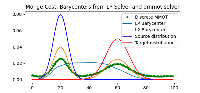
When the cost is discretized (Monge), the d-MMOT solver can more quickly compute and minimize the distance between many distributions without the need for intermediate barycenter computations. This example compares the time to identify, and the quality of, solutions for the d-MMOT problem using a primal/dual algorithm and classical LP barycenter approaches.
# Author: Ronak Mehta <ronakrm@cs.wisc.edu>
#         Xizheng Yu <xyu354@wisc.edu>
#
# License: MIT License

# sphinx_gallery_thumbnail_number = 2
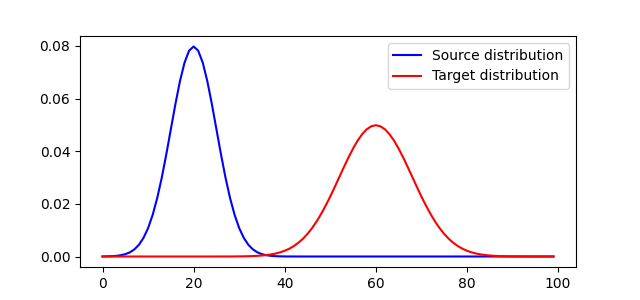
Generating 2 distributions
import numpy as np
import matplotlib.pyplot as pl
import ot

np.random.seed(0)

n = 100
d = 2
# Gaussian distributions
a1 = ot.datasets.make_1D_gauss(n, m=20, s=5)  # m=mean, s=std
a2 = ot.datasets.make_1D_gauss(n, m=60, s=8)
A = np.vstack((a1, a2)).T
x = np.arange(n, dtype=np.float64)
M = ot.utils.dist(x.reshape((n, 1)), metric="minkowski")

pl.figure(1, figsize=(6.4, 3))
pl.plot(x, a1, "b", label="Source distribution")
pl.plot(x, a2, "r", label="Target distribution")
pl.legend()
<matplotlib.legend.Legend object at 0x701d1dd984a0>
Minimize the distances among distributions, identify the Barycenter
The objective being minimized is different for both methods, so the objective values cannot be compared.
# L2 Iteration
weights = np.ones(d) / d
l2_bary = A.dot(weights)

print("LP Iterations:")
weights = np.ones(d) / d
lp_bary, lp_log = ot.lp.barycenter(
    A, M, weights, solver="interior-point", verbose=False, log=True
)
print("Time\t: ", ot.toc(""))
print("Obj\t: ", lp_log["fun"])

print("")
print("Discrete MMOT Algorithm:")
ot.tic()
barys, log = ot.lp.dmmot_monge_1dgrid_optimize(
    A, niters=4000, lr_init=1e-5, lr_decay=0.997, log=True
)
dmmot_obj = log["primal objective"]
print("Time\t: ", ot.toc(""))
print("Obj\t: ", dmmot_obj)
LP Iterations:
/home/circleci/project/ot/lp/_barycenter_solvers.py:132: OptimizeWarning: Sparse constraint matrix detected; setting 'sparse':True.
  sol = sp.optimize.linprog(

Time    :  84.47398587800035
Obj     :  19.999774737592773

Discrete MMOT Algorithm:
Initial:                Obj:    39.9995 GradNorm:       739.7831
Iter  0:        Obj:    39.9995 GradNorm:       739.7831
Iter 100:       Obj:    2.0914  GradNorm:       180.6322
Iter 200:       Obj:    1.0583  GradNorm:       434.3777
Iter 300:       Obj:    0.4220  GradNorm:       252.9269
Iter 400:       Obj:    0.2317  GradNorm:       168.8668
Iter 500:       Obj:    0.2116  GradNorm:       384.2968
Iter 600:       Obj:    0.1755  GradNorm:       647.6758
Iter 700:       Obj:    0.1343  GradNorm:       786.2442
Iter 800:       Obj:    0.1021  GradNorm:       810.3703
Iter 900:       Obj:    0.0662  GradNorm:       810.3703
Iter 1000:      Obj:    0.0539  GradNorm:       741.7304
Iter 1100:      Obj:    0.0348  GradNorm:       621.4660
Iter 1200:      Obj:    0.0338  GradNorm:       764.3429
Iter 1300:      Obj:    0.0200  GradNorm:       556.2338
Iter 1400:      Obj:    0.0182  GradNorm:       765.8329
Iter 1500:      Obj:    0.0103  GradNorm:       579.8241
Iter 1600:      Obj:    0.0075  GradNorm:       638.2570
Iter 1700:      Obj:    0.0045  GradNorm:       320.1562
Iter 1800:      Obj:    0.0035  GradNorm:       479.8625
Iter 1900:      Obj:    0.0032  GradNorm:       647.1939
Iter 2000:      Obj:    0.0022  GradNorm:       442.4975
Iter 2100:      Obj:    0.0015  GradNorm:       61.0901
Iter 2200:      Obj:    0.0016  GradNorm:       464.9430
Iter 2300:      Obj:    0.0014  GradNorm:       382.5650
Iter 2400:      Obj:    0.0011  GradNorm:       287.2281
Iter 2500:      Obj:    0.0011  GradNorm:       355.6796
Iter 2600:      Obj:    0.0010  GradNorm:       280.1357
Iter 2700:      Obj:    0.0010  GradNorm:       289.6964
Iter 2800:      Obj:    0.0010  GradNorm:       184.4234
Iter 2900:      Obj:    0.0009  GradNorm:       246.5847
Iter 3000:      Obj:    0.0009  GradNorm:       65.3299
Iter 3100:      Obj:    0.0009  GradNorm:       185.9355
Iter 3200:      Obj:    0.0009  GradNorm:       263.0209
Iter 3300:      Obj:    0.0009  GradNorm:       300.3132
Iter 3400:      Obj:    0.0009  GradNorm:       231.4044
Iter 3500:      Obj:    0.0009  GradNorm:       226.3184
Iter 3600:      Obj:    0.0009  GradNorm:       211.4237
Iter 3700:      Obj:    0.0009  GradNorm:       233.2981
Iter 3800:      Obj:    0.0009  GradNorm:       299.0853
Iter 3900:      Obj:    0.0009  GradNorm:       262.4271

Time    :  5.180457368000134
Obj     :  0.0008940778156521405
Compare Barycenters in both methods
pl.figure(1, figsize=(6.4, 3))
for i in range(len(barys)):
    if i == 0:
        pl.plot(x, barys[i], "g-*", label="Discrete MMOT")
    else:
        continue
        # pl.plot(x, barys[i], 'g-*')
pl.plot(x, lp_bary, label="LP Barycenter")
pl.plot(x, l2_bary, label="L2 Barycenter")
pl.plot(x, a1, "b", label="Source distribution")
pl.plot(x, a2, "r", label="Target distribution")
pl.title("Monge Cost: Barycenters from LP Solver and dmmot solver")
pl.legend()
<matplotlib.legend.Legend object at 0x701d3fe36ff0>
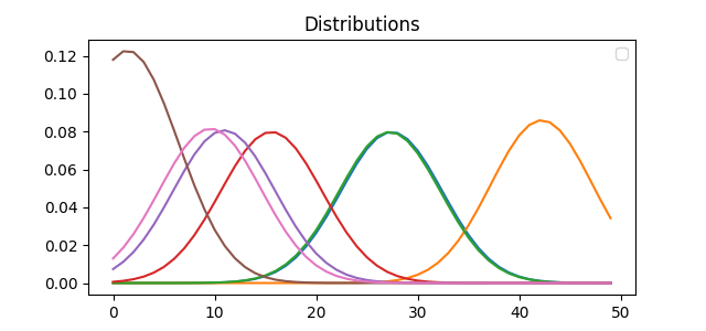
More than 2 distributions
Generate 7 pseudorandom gaussian distributions with 50 bins.
n = 50  # nb bins
d = 7
vecsize = n * d

data = []
for i in range(d):
    m = n * (0.5 * np.random.rand(1)) * float(np.random.randint(2) + 1)
    a = ot.datasets.make_1D_gauss(n, m=m, s=5)
    data.append(a)

x = np.arange(n, dtype=np.float64)
M = ot.utils.dist(x.reshape((n, 1)), metric="minkowski")
A = np.vstack(data).T

pl.figure(1, figsize=(6.4, 3))
for i in range(len(data)):
    pl.plot(x, data[i])

pl.title("Distributions")
pl.legend()
/home/circleci/project/examples/others/plot_dmmot.py:116: UserWarning: No artists with labels found to put in legend.  Note that artists whose label start with an underscore are ignored when legend() is called with no argument.
  pl.legend()

<matplotlib.legend.Legend object at 0x701d0941ec30>
Minimizing Distances Among Many Distributions
The objective being minimized is different for both methods, so the objective values cannot be compared.
# Perform gradient descent optimization using the d-MMOT method.
barys = ot.lp.dmmot_monge_1dgrid_optimize(A, niters=3000, lr_init=1e-4, lr_decay=0.997)

# after minimization, any distribution can be used as a estimate of barycenter.
bary = barys[0]

# Compute 1D Wasserstein barycenter using the L2/LP method
weights = ot.unif(d)
l2_bary = A.dot(weights)
lp_bary, bary_log = ot.lp.barycenter(
    A, M, weights, solver="interior-point", verbose=False, log=True
)
Initial:                Obj:    37.1964 GradNorm:       284.3413
Iter  0:        Obj:    37.1964 GradNorm:       280.9858
Iter 100:       Obj:    3.2628  GradNorm:       143.1922
Iter 200:       Obj:    0.8687  GradNorm:       165.7830
Iter 300:       Obj:    0.4563  GradNorm:       235.9619
Iter 400:       Obj:    0.3789  GradNorm:       253.4285
Iter 500:       Obj:    0.3109  GradNorm:       284.3413
Iter 600:       Obj:    0.2467  GradNorm:       284.3413
Iter 700:       Obj:    0.1794  GradNorm:       284.3413
Iter 800:       Obj:    0.1023  GradNorm:       262.5719
Iter 900:       Obj:    0.0815  GradNorm:       276.6912
Iter 1000:      Obj:    0.0575  GradNorm:       258.2634
Iter 1100:      Obj:    0.0450  GradNorm:       233.6365
Iter 1200:      Obj:    0.0292  GradNorm:       218.8698
Iter 1300:      Obj:    0.0264  GradNorm:       262.0572
Iter 1400:      Obj:    0.0161  GradNorm:       212.5559
Iter 1500:      Obj:    0.0132  GradNorm:       231.8016
Iter 1600:      Obj:    0.0091  GradNorm:       193.5355
Iter 1700:      Obj:    0.0069  GradNorm:       195.1973
Iter 1800:      Obj:    0.0053  GradNorm:       186.4350
Iter 1900:      Obj:    0.0043  GradNorm:       184.0869
Iter 2000:      Obj:    0.0035  GradNorm:       195.0077
Iter 2100:      Obj:    0.0028  GradNorm:       157.2132
Iter 2200:      Obj:    0.0024  GradNorm:       169.3930
Iter 2300:      Obj:    0.0022  GradNorm:       161.6787
Iter 2400:      Obj:    0.0020  GradNorm:       147.3635
Iter 2500:      Obj:    0.0018  GradNorm:       162.9417
Iter 2600:      Obj:    0.0017  GradNorm:       144.6790
Iter 2700:      Obj:    0.0016  GradNorm:       164.0792
Iter 2800:      Obj:    0.0016  GradNorm:       121.3507
Iter 2900:      Obj:    0.0015  GradNorm:       150.1533
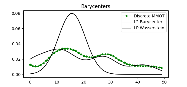
Compare Barycenters in both methods
<matplotlib.legend.Legend object at 0x701cfb3ac3e0>
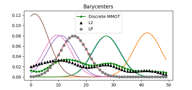
Compare with original distributions
pl.figure(1, figsize=(6.4, 3))
for i in range(len(data)):
    pl.plot(x, data[i])
for i in range(len(barys)):
    if i == 0:
        pl.plot(x, barys[i], "g-*", label="Discrete MMOT")
    else:
        continue
        # pl.plot(x, barys[i], 'g')
pl.plot(x, l2_bary, "k^", label="L2")
pl.plot(x, lp_bary, "o", color="grey", label="LP")
pl.title("Barycenters")
pl.legend()
pl.show()
Total running time of the script: (0 minutes 29.232 seconds)