Weak Optimal Transport VS exact Optimal Transport

Note

Example added in release: 0.8.2.

Illustration of 2D optimal transport between distributions that are weighted sum of Diracs. The OT matrix is plotted with the samples.

# Author: Remi Flamary <remi.flamary@polytechnique.edu>
#
# License: MIT License

# sphinx_gallery_thumbnail_number = 4

import numpy as np
import matplotlib.pylab as pl
import ot
import ot.plot

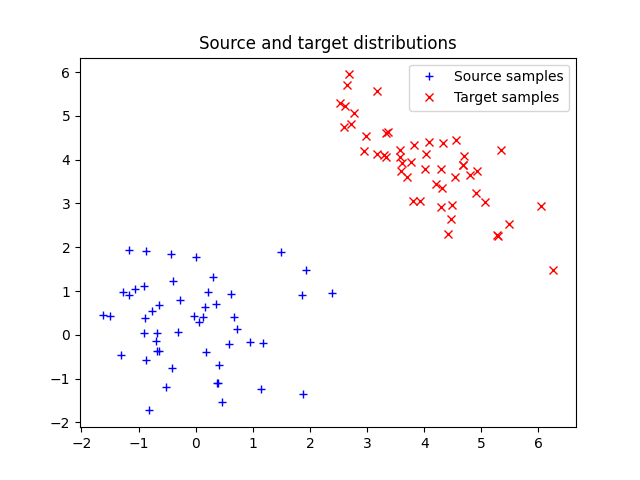
Generate data an plot it

n = 50  # nb samples

mu_s = np.array([0, 0])
cov_s = np.array([[1, 0], [0, 1]])

mu_t = np.array([4, 4])
cov_t = np.array([[1, -0.8], [-0.8, 1]])

xs = ot.datasets.make_2D_samples_gauss(n, mu_s, cov_s)
xt = ot.datasets.make_2D_samples_gauss(n, mu_t, cov_t)

a, b = ot.unif(n), ot.unif(n)  # uniform distribution on samples

# loss matrix
M = ot.dist(xs, xt)
M /= M.max()

pl.figure(1)
pl.plot(xs[:, 0], xs[:, 1], "+b", label="Source samples")
pl.plot(xt[:, 0], xt[:, 1], "xr", label="Target samples")
pl.legend(loc=0)
pl.title("Source and target distributions")

pl.figure(2)
pl.imshow(M, interpolation="nearest")
pl.title("Cost matrix M")

• 
• 

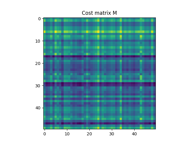
Text(0.5, 1.0, 'Cost matrix M')

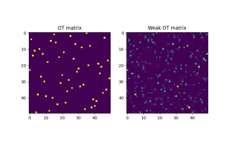
Compute Weak OT and exact OT solutions

G0 = ot.emd(a, b, M)

Gweak = ot.weak_optimal_transport(xs, xt, a, b)

Plot weak OT and exact OT solutions

pl.figure(3, (8, 5))

pl.subplot(1, 2, 1)
pl.imshow(G0, interpolation="nearest")
pl.title("OT matrix")

pl.subplot(1, 2, 2)
pl.imshow(Gweak, interpolation="nearest")
pl.title("Weak OT matrix")

pl.figure(4, (8, 5))

pl.subplot(1, 2, 1)
ot.plot.plot2D_samples_mat(xs, xt, G0, c=[0.5, 0.5, 1])
pl.plot(xs[:, 0], xs[:, 1], "+b", label="Source samples")
pl.plot(xt[:, 0], xt[:, 1], "xr", label="Target samples")
pl.title("OT matrix with samples")

pl.subplot(1, 2, 2)
ot.plot.plot2D_samples_mat(xs, xt, Gweak, c=[0.5, 0.5, 1])
pl.plot(xs[:, 0], xs[:, 1], "+b", label="Source samples")
pl.plot(xt[:, 0], xt[:, 1], "xr", label="Target samples")
pl.title("Weak OT matrix with samples")

• 
• 

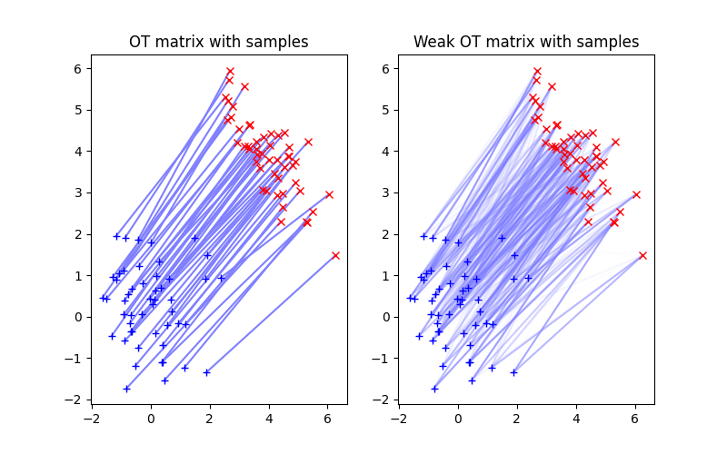
Text(0.5, 1.0, 'Weak OT matrix with samples')