GMM Plan 1D

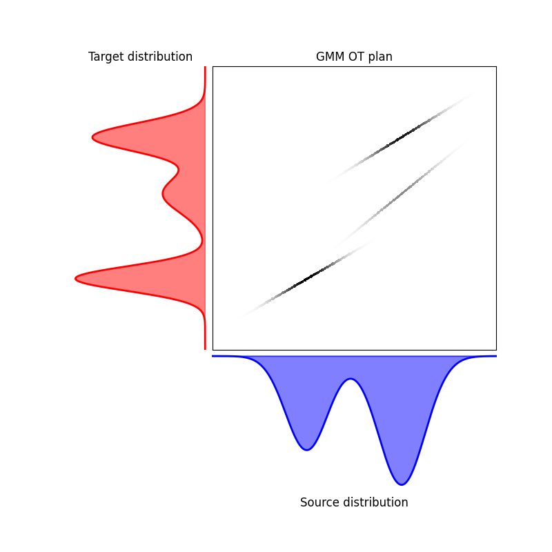
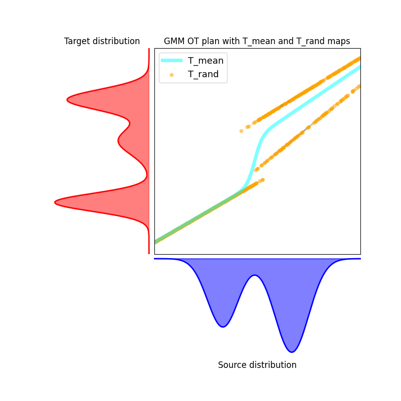
Illustration of the GMM plan for the Mixture Wasserstein between two GMM in 1D, as well as the two maps T_mean and T_rand. T_mean is the barycentric projection of the GMM coupling, and T_rand takes a random gaussian image between two components, according to the coupling and the GMMs. See [69] for details. .. [69] Delon, J., & Desolneux, A. (2020). A Wasserstein-type distance in the space of Gaussian mixture models. SIAM Journal on Imaging Sciences, 13(2), 936-970.

# Author: Eloi Tanguy <eloi.tanguy@u-paris>
#         Remi Flamary <remi.flamary@polytehnique.edu>
#         Julie Delon <julie.delon@math.cnrs.fr>
#
# License: MIT License

# sphinx_gallery_thumbnail_number = 1

import numpy as np
from ot.plot import plot1D_mat, rescale_for_imshow_plot
from ot.gmm import gmm_ot_plan_density, gmm_pdf, gmm_ot_apply_map
import matplotlib.pyplot as plt

Generate GMMOT plan plot it

ks = 2
kt = 3
d = 1
eps = 0.1
m_s = np.array([[1], [2]])
m_t = np.array([[3], [4.2], [5]])
C_s = np.array([[[0.05]], [[0.06]]])
C_t = np.array([[[0.03]], [[0.07]], [[0.04]]])
w_s = np.array([0.4, 0.6])
w_t = np.array([0.4, 0.2, 0.4])

n = 500
a_x, b_x = 0, 3
x = np.linspace(a_x, b_x, n)
a_y, b_y = 2, 6
y = np.linspace(a_y, b_y, n)
plan_density = gmm_ot_plan_density(
    x[:, None], y[:, None], m_s, m_t, C_s, C_t, w_s, w_t, plan=None, atol=2e-2
)

a = gmm_pdf(x[:, None], m_s, C_s, w_s)
b = gmm_pdf(y[:, None], m_t, C_t, w_t)
plt.figure(figsize=(8, 8))
plot1D_mat(
    a,
    b,
    plan_density,
    title="GMM OT plan",
    plot_style="xy",
    a_label="Source distribution",
    b_label="Target distribution",
)

(<Axes: title={'center': 'Source distribution'}>, <Axes: title={'center': 'Target distribution'}>, <Axes: title={'center': 'GMM OT plan'}>)

Generate GMMOT maps and plot them over plan

plt.figure(figsize=(8, 8))
ax_s, ax_t, ax_M = plot1D_mat(
    a,
    b,
    plan_density,
    plot_style="xy",
    title="GMM OT plan with T_mean and T_rand maps",
    a_label="Source distribution",
    b_label="Target distribution",
)
T_mean = gmm_ot_apply_map(x[:, None], m_s, m_t, C_s, C_t, w_s, w_t, method="bary")[:, 0]
x_rescaled, T_mean_rescaled = rescale_for_imshow_plot(x, T_mean, n, a_y=a_y, b_y=b_y)

ax_M.plot(
    x_rescaled, T_mean_rescaled, label="T_mean", alpha=0.5, linewidth=5, color="aqua"
)

T_rand = gmm_ot_apply_map(
    x[:, None], m_s, m_t, C_s, C_t, w_s, w_t, method="rand", seed=0
)[:, 0]
x_rescaled, T_rand_rescaled = rescale_for_imshow_plot(x, T_rand, n, a_y=a_y, b_y=b_y)

ax_M.scatter(
    x_rescaled, T_rand_rescaled, label="T_rand", alpha=0.5, s=20, color="orange"
)

ax_M.legend(loc="upper left", fontsize=13)

<matplotlib.legend.Legend object at 0x7626441e44c0>