Wasserstein Discriminant Analysis

Note

Example added in release: 0.3.0.

This example illustrate the use of WDA as proposed in [11].

[11] Flamary, R., Cuturi, M., Courty, N., & Rakotomamonjy, A. (2016). Wasserstein Discriminant Analysis.

# Author: Remi Flamary <remi.flamary@unice.fr>
#
# License: MIT License

# sphinx_gallery_thumbnail_number = 2

import numpy as np
import matplotlib.pylab as pl

from ot.dr import wda, fda

Generate data

n = 1000  # nb samples in source and target datasets
nz = 0.2

np.random.seed(1)

# generate circle dataset
t = np.random.rand(n) * 2 * np.pi
ys = np.floor((np.arange(n) * 1.0 / n * 3)) + 1
xs = np.concatenate((np.cos(t).reshape((-1, 1)), np.sin(t).reshape((-1, 1))), 1)
xs = xs * ys.reshape(-1, 1) + nz * np.random.randn(n, 2)

t = np.random.rand(n) * 2 * np.pi
yt = np.floor((np.arange(n) * 1.0 / n * 3)) + 1
xt = np.concatenate((np.cos(t).reshape((-1, 1)), np.sin(t).reshape((-1, 1))), 1)
xt = xt * yt.reshape(-1, 1) + nz * np.random.randn(n, 2)

nbnoise = 8

xs = np.hstack((xs, np.random.randn(n, nbnoise)))
xt = np.hstack((xt, np.random.randn(n, nbnoise)))

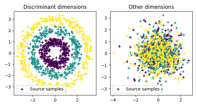
Plot data

pl.figure(1, figsize=(6.4, 3.5))

pl.subplot(1, 2, 1)
pl.scatter(xt[:, 0], xt[:, 1], c=ys, marker="+", label="Source samples")
pl.legend(loc=0)
pl.title("Discriminant dimensions")

pl.subplot(1, 2, 2)
pl.scatter(xt[:, 2], xt[:, 3], c=ys, marker="+", label="Source samples")
pl.legend(loc=0)
pl.title("Other dimensions")
pl.tight_layout()

Compute Fisher Discriminant Analysis

p = 2

Pfda, projfda = fda(xs, ys, p)

Compute Wasserstein Discriminant Analysis

p = 2
reg = 1e0
k = 10
maxiter = 100

P0 = np.random.randn(xs.shape[1], p)

P0 /= np.sqrt(np.sum(P0**2, 0, keepdims=True))

Pwda, projwda = wda(xs, ys, p, reg, k, maxiter=maxiter, P0=P0)

Optimizing...
Iteration    Cost                       Gradient norm
---------    -----------------------    --------------
  1          +8.3042776946697483e-01    5.65147154e-01
  2          +4.4401037686381040e-01    2.16760501e-01
  3          +4.2234351238819928e-01    1.30555049e-01
  4          +4.2169879996364479e-01    1.39115407e-01
  5          +4.1924746118060674e-01    1.25387848e-01
  6          +4.1177409528990933e-01    6.70993539e-02
  7          +4.0862213476139003e-01    3.52716830e-02
  8          +4.0747229322240336e-01    3.34923131e-02
  9          +4.0678766065261329e-01    2.74029183e-02
 10          +4.0621337155459925e-01    2.03651803e-02
 11          +4.0577080390746961e-01    2.59605592e-02
 12          +4.0543140912477149e-01    3.28883715e-02
 13          +4.0470236926311942e-01    1.47528039e-02
 14          +4.0445628467113731e-01    5.03183253e-02
 15          +4.0364189454514843e-01    3.31006501e-02
 16          +4.0303977564978699e-01    1.39885362e-02
 17          +4.0301476232780259e-01    2.17467590e-02
 18          +4.0292344279343950e-01    1.79959771e-02
 19          +4.0271888307907128e-01    6.94408749e-03
 20          +4.0183215737046896e-01    1.98326640e-02
 21          +3.9762707100593531e-01    1.03195400e-01
 22          +3.8225988079706485e-01    1.35998904e-01
 23          +3.0856544070652298e-01    1.92703391e-01
 24          +2.7998481492927213e-01    2.01878706e-01
 25          +2.3693225637656293e-01    9.05665571e-02
 26          +2.3416660805509620e-01    7.09781011e-02
 27          +2.3173761386491401e-01    4.03937487e-02
 28          +2.3061384109180777e-01    3.70147365e-03
 29          +2.3061161834370525e-01    3.25958826e-03
 30          +2.3060547914991694e-01    1.24366264e-03
 31          +2.3060465305946115e-01    5.78888734e-04
 32          +2.3060458219792498e-01    4.79935562e-04
 33          +2.3060442824951685e-01    4.16489862e-05
 34          +2.3060442707775350e-01    1.55904146e-06
 35          +2.3060442707614406e-01    5.08692969e-07
Terminated - min grad norm reached after 35 iterations, 5.21 seconds.

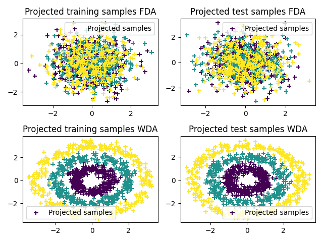
Plot 2D projections

xsp = projfda(xs)
xtp = projfda(xt)

xspw = projwda(xs)
xtpw = projwda(xt)

pl.figure(2)

pl.subplot(2, 2, 1)
pl.scatter(xsp[:, 0], xsp[:, 1], c=ys, marker="+", label="Projected samples")
pl.legend(loc=0)
pl.title("Projected training samples FDA")

pl.subplot(2, 2, 2)
pl.scatter(xtp[:, 0], xtp[:, 1], c=ys, marker="+", label="Projected samples")
pl.legend(loc=0)
pl.title("Projected test samples FDA")

pl.subplot(2, 2, 3)
pl.scatter(xspw[:, 0], xspw[:, 1], c=ys, marker="+", label="Projected samples")
pl.legend(loc=0)
pl.title("Projected training samples WDA")

pl.subplot(2, 2, 4)
pl.scatter(xtpw[:, 0], xtpw[:, 1], c=ys, marker="+", label="Projected samples")
pl.legend(loc=0)
pl.title("Projected test samples WDA")
pl.tight_layout()

pl.show()

/home/circleci/.local/lib/python3.12/site-packages/matplotlib/cbook.py:1810: ComplexWarning: Casting complex values to real discards the imaginary part
  return math.isfinite(val)
/home/circleci/.local/lib/python3.12/site-packages/matplotlib/collections.py:205: ComplexWarning: Casting complex values to real discards the imaginary part
  offsets = np.asanyarray(offsets, float)