Note
Go to the end to download the full example code.
Learning sample marginal distribution with CO-Optimal Transport
In this example, we illustrate how to estimate the sample marginal distribution which minimizes the CO-Optimal Transport distance [47]_ between two matrices. More precisely, given a source data \((X, \mu_x^{(s)}, \mu_x^{(f)})\) and a target matrix \(Y\) associated with a fixed histogram on features \(\mu_y^{(f)}\), we want to solve the following problem
where \(\Delta\) is the probability simplex. This minimization is done with a
simple projected gradient descent in PyTorch. We use the automatic backend of POT that
allows us to compute the CO-Optimal Transport distance with ot.coot.co_optimal_transport2()
with differentiable losses.
# Author: Remi Flamary <remi.flamary@unice.fr>
#         Quang Huy Tran <quang-huy.tran@univ-ubs.fr>
# License: MIT License

from matplotlib.patches import ConnectionPatch
import torch
import numpy as np

import matplotlib.pyplot as pl
import ot

from ot.coot import co_optimal_transport as coot
from ot.coot import co_optimal_transport2 as coot2
Generate data
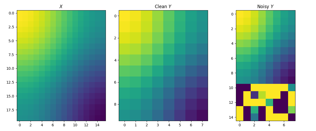
The source and clean target matrices are generated by \(X_{i,j} = \cos(\frac{i}{n_1} \pi) + \cos(\frac{j}{d_1} \pi)\) and \(Y_{i,j} = \cos(\frac{i}{n_2} \pi) + \cos(\frac{j}{d_2} \pi)\). The target matrix is then contaminated by adding 5 row outliers. Intuitively, we expect that the estimated sample distribution should ignore these outliers, i.e. their weights should be zero.
np.random.seed(182)

n1, d1 = 20, 16
n2, d2 = 10, 8
n = 15

X = (
    torch.cos(torch.arange(n1) * torch.pi / n1)[:, None] +
    torch.cos(torch.arange(d1) * torch.pi / d1)[None, :]
)

# Generate clean target data mixed with outliers
Y_noisy = torch.randn((n, d2)) * 10.0
Y_noisy[:n2, :] = (
    torch.cos(torch.arange(n2) * torch.pi / n2)[:, None] +
    torch.cos(torch.arange(d2) * torch.pi / d2)[None, :]
)
Y = Y_noisy[:n2, :]

X, Y_noisy, Y = X.double(), Y_noisy.double(), Y.double()

fig, axes = pl.subplots(nrows=1, ncols=3, figsize=(12, 5))
axes[0].imshow(X, vmin=-2, vmax=2)
axes[0].set_title('$X$')

axes[1].imshow(Y, vmin=-2, vmax=2)
axes[1].set_title('Clean $Y$')

axes[2].imshow(Y_noisy, vmin=-2, vmax=2)
axes[2].set_title('Noisy $Y$')

pl.tight_layout()
Optimize the COOT distance with respect to the sample marginal distribution
losses = []
lr = 1e-3
niter = 1000

b = torch.tensor(ot.unif(n), requires_grad=True)

for i in range(niter):

    loss = coot2(X, Y_noisy, wy_samp=b, log=False, verbose=False)
    losses.append(float(loss))

    loss.backward()

    with torch.no_grad():
        b -= lr * b.grad  # gradient step
        b[:] = ot.utils.proj_simplex(b)  # projection on the simplex

    b.grad.zero_()

# Estimated sample marginal distribution and training loss curve
pl.plot(losses[10:])
pl.title('CO-Optimal Transport distance')

print(f"Marginal distribution = {b.detach().numpy()}")
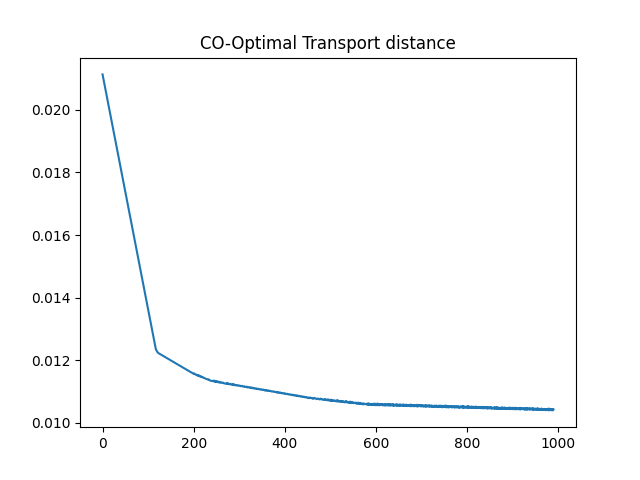
Marginal distribution = [0.07507868 0.08001347 0.09469872 0.1001999  0.10001527 0.10001687
 0.09999904 0.09979829 0.11466591 0.13551386 0.         0.
 0.         0.         0.        ]
Visualizing the row and column alignments with the estimated sample marginal distribution
Clearly, the learned marginal distribution completely and successfully ignores the 5 outliers.
X, Y_noisy = X.numpy(), Y_noisy.numpy()
b = b.detach().numpy()

pi_sample, pi_feature = coot(X, Y_noisy, wy_samp=b, log=False, verbose=True)

fig = pl.figure(4, (9, 7))
pl.clf()

ax1 = pl.subplot(2, 2, 3)
pl.imshow(X, vmin=-2, vmax=2)
pl.xlabel('$X$')

ax2 = pl.subplot(2, 2, 2)
ax2.yaxis.tick_right()
pl.imshow(np.transpose(Y_noisy), vmin=-2, vmax=2)
pl.title("Transpose(Noisy $Y$)")
ax2.xaxis.tick_top()

for i in range(n1):
    j = np.argmax(pi_sample[i, :])
    xyA = (d1 - .5, i)
    xyB = (j, d2 - .5)
    con = ConnectionPatch(xyA=xyA, xyB=xyB, coordsA=ax1.transData,
                          coordsB=ax2.transData, color="black")
    fig.add_artist(con)

for i in range(d1):
    j = np.argmax(pi_feature[i, :])
    xyA = (i, -.5)
    xyB = (-.5, j)
    con = ConnectionPatch(
        xyA=xyA, xyB=xyB, coordsA=ax1.transData, coordsB=ax2.transData, color="blue")
    fig.add_artist(con)
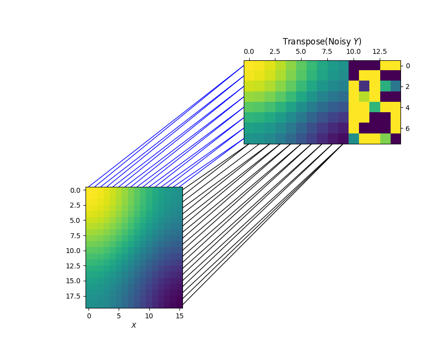
CO-Optimal Transport cost at iteration 1: 0.010389716046318498
Total running time of the script: (0 minutes 3.856 seconds)