Quantized Fused Gromov-Wasserstein examples

These examples show how to use the quantized (Fused) Gromov-Wasserstein solvers (qFGW) [68]. POT provides a generic solver quantized_fused_gromov_wasserstein_partitioned that takes as inputs partitioned graphs potentially endowed with node features, which have to be built by the user. On top of that, POT provides two wrappers:

i) quantized_fused_gromov_wasserstein operating over generic graphs, whose partitioning is performed via get_graph_partition using e.g the Louvain algorithm, and representant for each partition can be selected via get_graph_representants using e.g the PageRank algorithm.

ii) quantized_fused_gromov_wasserstein_samples operating over point clouds, e.g \(X_1 \in R^{n_1 * d_1}\) and \(X_2 \in R^{n_2 * d_2}\) endowed with their respective euclidean geometry, whose partitioning and representant selection is performed jointly using e.g the K-means algorithm via the function get_partition_and_representants_samples.

We illustrate next how to compute the qGW distance on both types of data by:

i) Generating two graphs following Stochastic Block Models encoded as shortest path matrices as qGW solvers tends to require dense structure to achieve a good approximation of the GW distance (as qGW is an upper-bound of GW). In the meantime, we illustrate an optional feature of our solvers, namely the use of auxiliary structures e.g adjacency matrices to perform the graph partitioning.

ii) Generating two point clouds representing curves in 2D and 3D respectively. We augment these point clouds by considering additional features of the same dimensionaly \(F_1 \in R^{n_1 * d}\) and \(F_2 \in R^{n_2 * d}\), representing the color intensity associated to each sample of both distributions. Then we compute the qFGW distance between these attributed point clouds.

[68] Chowdhury, S., Miller, D., & Needham, T. (2021). Quantized gromov-wasserstein. ECML PKDD 2021. Springer International Publishing.

# Author: Cédric Vincent-Cuaz <cedvincentcuaz@gmail.com>
#
# License: MIT License

# sphinx_gallery_thumbnail_number = 2

import numpy as np
import matplotlib.pylab as pl
import matplotlib.pyplot as plt
import networkx
from networkx.generators.community import stochastic_block_model as sbm
from scipy.sparse.csgraph import shortest_path

from ot.gromov import (
    quantized_fused_gromov_wasserstein_partitioned, quantized_fused_gromov_wasserstein,
    get_graph_partition, get_graph_representants, format_partitioned_graph,
    quantized_fused_gromov_wasserstein_samples,
    get_partition_and_representants_samples)

Generate graphs

Create two graphs following Stochastic Block models of 2 and 3 clusters.

N1 = 30  # 2 communities
N2 = 45  # 3 communities
p1 = [[0.8, 0.1],
      [0.1, 0.7]]
p2 = [[0.8, 0.1, 0.],
      [0.1, 0.75, 0.1],
      [0., 0.1, 0.7]]
G1 = sbm(seed=0, sizes=[N1 // 2, N1 // 2], p=p1)
G2 = sbm(seed=0, sizes=[N2 // 3, N2 // 3, N2 // 3], p=p2)


C1 = networkx.to_numpy_array(G1)
C2 = networkx.to_numpy_array(G2)

spC1 = shortest_path(C1)
spC2 = shortest_path(C2)

h1 = np.ones(C1.shape[0]) / C1.shape[0]
h2 = np.ones(C2.shape[0]) / C2.shape[0]

# Add weights on the edges for visualization later on
weight_intra_G1 = 5
weight_inter_G1 = 0.5
weight_intra_G2 = 1.
weight_inter_G2 = 1.5

weightedG1 = networkx.Graph()
part_G1 = [G1.nodes[i]['block'] for i in range(N1)]

for node in G1.nodes():
    weightedG1.add_node(node)
for i, j in G1.edges():
    if part_G1[i] == part_G1[j]:
        weightedG1.add_edge(i, j, weight=weight_intra_G1)
    else:
        weightedG1.add_edge(i, j, weight=weight_inter_G1)

weightedG2 = networkx.Graph()
part_G2 = [G2.nodes[i]['block'] for i in range(N2)]

for node in G2.nodes():
    weightedG2.add_node(node)
for i, j in G2.edges():
    if part_G2[i] == part_G2[j]:
        weightedG2.add_edge(i, j, weight=weight_intra_G2)
    else:
        weightedG2.add_edge(i, j, weight=weight_inter_G2)


# setup for graph visualization

def node_coloring(part, starting_color=0):

    # get graphs partition and their coloring
    unique_colors = ['C%s' % (starting_color + i) for i in np.unique(part)]
    nodes_color_part = []
    for cluster in part:
        nodes_color_part.append(unique_colors[cluster])

    return nodes_color_part


def draw_graph(G, C, nodes_color_part, rep_indices, node_alphas=None, pos=None,
               edge_color='black', alpha_edge=0.7, node_size=None,
               shiftx=0, seed=0, highlight_rep=False):

    if (pos is None):
        pos = networkx.spring_layout(G, scale=1., seed=seed)

    if shiftx != 0:
        for k, v in pos.items():
            v[0] = v[0] + shiftx

    width_edge = 1.5

    if not highlight_rep:
        networkx.draw_networkx_edges(
            G, pos, width=width_edge, alpha=alpha_edge, edge_color=edge_color)
    else:
        for edge in G.edges:
            if (edge[0] in rep_indices) and (edge[1] in rep_indices):
                networkx.draw_networkx_edges(
                    G, pos, edgelist=[edge], width=width_edge, alpha=alpha_edge,
                    edge_color=edge_color)
            else:
                networkx.draw_networkx_edges(
                    G, pos, edgelist=[edge], width=width_edge, alpha=0.2,
                    edge_color=edge_color)

    for node, node_color in enumerate(nodes_color_part):
        local_node_shape, local_node_size = 'o', node_size

        if highlight_rep:
            if node in rep_indices:
                local_node_shape, local_node_size = '*', 6 * node_size

        if node_alphas is None:
            alpha = 0.9
            if highlight_rep:
                alpha = 0.9 if node in rep_indices else 0.1

        else:
            alpha = node_alphas[node]

        networkx.draw_networkx_nodes(G, pos, nodelist=[node], alpha=alpha,
                                     node_shape=local_node_shape,
                                     node_size=local_node_size,
                                     node_color=node_color)

    return pos

Compute their quantized Gromov-Wasserstein distance without using the wrapper

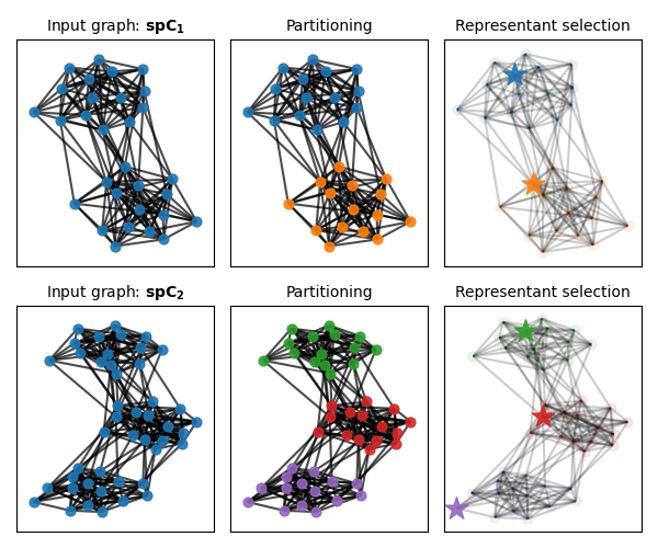
We detail next the steps implemented within the wrapper that preprocess graphs to form partitioned graphs, which are then passed as input to the generic qFGW solver.

# 1-a) Partition C1 and C2 in 2 and 3 clusters respectively using Louvain
#    algorithm from Networkx. Then encode these partitions via vectors of assignments.

part_method = 'louvain'
rep_method = 'pagerank'

npart_1 = 2  # 2 clusters used to describe C1
npart_2 = 3  # 3 clusters used to describe C2

part1 = get_graph_partition(
    C1, npart=npart_1, part_method=part_method, F=None, alpha=1.)
part2 = get_graph_partition(
    C2, npart=npart_2, part_method=part_method, F=None, alpha=1.)

# 1-b) Select representant in each partition using the Pagerank algorithm
#     implementation from networkx.

rep_indices1 = get_graph_representants(C1, part1, rep_method=rep_method)
rep_indices2 = get_graph_representants(C2, part2, rep_method=rep_method)

# 1-c) Formate partitions such that:
# CR contains relations between representants in each space.
# list_R contains relations between samples and representants within each partition.
# list_h contains samples relative importance within each partition.

CR1, list_R1, list_h1 = format_partitioned_graph(
    spC1, h1, part1, rep_indices1, F=None, M=None, alpha=1.)

CR2, list_R2, list_h2 = format_partitioned_graph(
    spC2, h2, part2, rep_indices2, F=None, M=None, alpha=1.)

# 1-d) call to partitioned quantized gromov-wasserstein solver

OT_global_, OTs_local_, OT_, log_ = quantized_fused_gromov_wasserstein_partitioned(
    CR1, CR2, list_R1, list_R2, list_h1, list_h2, MR=None,
    alpha=1., build_OT=True, log=True)


# Visualization of the graph pre-processing

node_size = 40
fontsize = 10
seed_G1 = 0
seed_G2 = 3

part1_ = part1.astype(np.int32)
part2_ = part2.astype(np.int32)


nodes_color_part1 = node_coloring(part1_, starting_color=0)
nodes_color_part2 = node_coloring(part2_, starting_color=np.unique(nodes_color_part1).shape[0])


pl.figure(1, figsize=(6, 5))
pl.clf()
pl.axis('off')
pl.subplot(2, 3, 1)
pl.title(r'Input graph: $\mathbf{spC_1}$', fontsize=fontsize)

pos1 = draw_graph(
    G1, C1, ['C0' for _ in part1_], rep_indices1, node_size=node_size, seed=seed_G1)

pl.subplot(2, 3, 2)
pl.title('Partitioning', fontsize=fontsize)

_ = draw_graph(
    G1, C1, nodes_color_part1, rep_indices1, pos=pos1, node_size=node_size, seed=seed_G1)

pl.subplot(2, 3, 3)
pl.title('Representant selection', fontsize=fontsize)

_ = draw_graph(
    G1, C1, nodes_color_part1, rep_indices1, pos=pos1, node_size=node_size,
    seed=seed_G1, highlight_rep=True)

pl.subplot(2, 3, 4)
pl.title(r'Input graph: $\mathbf{spC_2}$', fontsize=fontsize)

pos2 = draw_graph(
    G2, C2, ['C0' for _ in part2_], rep_indices2, node_size=node_size, seed=seed_G2)

pl.subplot(2, 3, 5)
pl.title(r'Partitioning', fontsize=fontsize)

_ = draw_graph(
    G2, C2, nodes_color_part2, rep_indices2, pos=pos2, node_size=node_size, seed=seed_G2)

pl.subplot(2, 3, 6)
pl.title(r'Representant selection', fontsize=fontsize)

_ = draw_graph(
    G2, C2, nodes_color_part2, rep_indices2, pos=pos2, node_size=node_size,
    seed=seed_G2, highlight_rep=True)
pl.tight_layout()

Compute the quantized Gromov-Wasserstein distance using the wrapper

Compute qGW(spC1, h1, spC2, h2). We also illustrate the use of auxiliary matrices such that the adjacency matrices C1_aux=C1 and C2_aux=C2 to partition the graph using Louvain algorithm, and the Pagerank algorithm for selecting representant within each partition. Notice that C1_aux and C2_aux are optional, if they are not specified these pre-processing algorithms will be applied to spC2 and spC3.

# no node features are considered on this synthetic dataset. Hence we simply
# let F1, F2 = None and set alpha = 1.
OT_global, OTs_local, OT, log = quantized_fused_gromov_wasserstein(
    spC1, spC2, npart_1, npart_2, h1, h2, C1_aux=C1, C2_aux=C2, F1=None, F2=None,
    alpha=1., part_method=part_method, rep_method=rep_method, log=True)

qGW_dist = log['qFGW_dist']

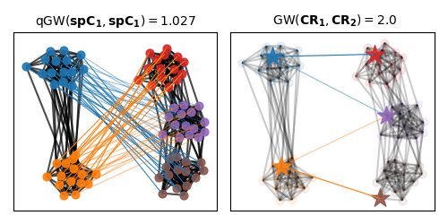
Visualization of the quantized Gromov-Wasserstein matching

We color nodes of the graph based on the respective partition of each graph. On the first plot we illustrate the qGW matching between both shortest path matrices. While the GW matching across representants of each space is illustrated on the right.

def draw_transp_colored_qGW(
        G1, C1, G2, C2, part1, part2, rep_indices1, rep_indices2, T,
        pos1=None, pos2=None, shiftx=4, switchx=False, node_size=70,
        seed_G1=0, seed_G2=0, highlight_rep=False):
    starting_color = 0
    # get graphs partition and their coloring
    unique_colors1 = ['C%s' % (starting_color + i) for i in np.unique(part1)]
    nodes_color_part1 = []
    for cluster in part1:
        nodes_color_part1.append(unique_colors1[cluster])

    starting_color = len(unique_colors1) + 1
    unique_colors2 = ['C%s' % (starting_color + i) for i in np.unique(part2)]
    nodes_color_part2 = []
    for cluster in part2:
        nodes_color_part2.append(unique_colors2[cluster])

    pos1 = draw_graph(
        G1, C1, nodes_color_part1, rep_indices1, pos=pos1, node_size=node_size,
        shiftx=0, seed=seed_G1, highlight_rep=highlight_rep)
    pos2 = draw_graph(
        G2, C2, nodes_color_part2, rep_indices2, pos=pos2, node_size=node_size,
        shiftx=shiftx, seed=seed_G1, highlight_rep=highlight_rep)

    if not highlight_rep:
        for k1, v1 in pos1.items():
            max_Tk1 = np.max(T[k1, :])
            for k2, v2 in pos2.items():
                if (T[k1, k2] > 0):
                    pl.plot([pos1[k1][0], pos2[k2][0]],
                            [pos1[k1][1], pos2[k2][1]],
                            '-', lw=0.7, alpha=T[k1, k2] / max_Tk1,
                            color=nodes_color_part1[k1])

    else:  # OT is only between representants
        for id1, node_id1 in enumerate(rep_indices1):
            max_Tk1 = np.max(T[id1, :])
            for id2, node_id2 in enumerate(rep_indices2):
                if (T[id1, id2] > 0):
                    pl.plot([pos1[node_id1][0], pos2[node_id2][0]],
                            [pos1[node_id1][1], pos2[node_id2][1]],
                            '-', lw=0.8, alpha=T[id1, id2] / max_Tk1,
                            color=nodes_color_part1[node_id1])
    return pos1, pos2


pl.figure(2, figsize=(5, 2.5))
pl.clf()
pl.axis('off')
pl.subplot(1, 2, 1)
pl.title(r'qGW$(\mathbf{spC_1}, \mathbf{spC_1}) =%s$' % (np.round(qGW_dist, 3)), fontsize=fontsize)

pos1, pos2 = draw_transp_colored_qGW(
    weightedG1, C1, weightedG2, C2, part1_, part2_, rep_indices1, rep_indices2,
    T=OT_, shiftx=1.5, node_size=node_size, seed_G1=seed_G1, seed_G2=seed_G2)

pl.tight_layout()

pl.subplot(1, 2, 2)
pl.title(r' GW$(\mathbf{CR_1}, \mathbf{CR_2}) =%s$' % (np.round(log_['global dist'], 3)), fontsize=fontsize)

pos1, pos2 = draw_transp_colored_qGW(
    weightedG1, C1, weightedG2, C2, part1_, part2_, rep_indices1, rep_indices2,
    T=OT_global, shiftx=1.5, node_size=node_size, seed_G1=seed_G1, seed_G2=seed_G2,
    highlight_rep=True)

pl.tight_layout()
pl.show()

Generate attributed point clouds

Create two attributed point clouds representing curves in 2D and 3D respectively, whose samples are further associated to various color intensities.

n_samples = 100

# Generate 2D and 3D curves
theta = np.linspace(-4 * np.pi, 4 * np.pi, n_samples)
z = np.linspace(1, 2, n_samples)
r = z**2 + 1
x = r * np.sin(theta)
y = r * np.cos(theta)

# Source and target distribution across spaces encoded respectively via their
# squared euclidean distance matrices.

X = np.concatenate([x.reshape(-1, 1), z.reshape(-1, 1)], axis=1)
Y = np.concatenate([x.reshape(-1, 1), y.reshape(-1, 1), z.reshape(-1, 1)], axis=1)

# Further associated to color intensity features derived from z

FX = z - z.min() / (z.max() - z.min())
FX = np.clip(0.8 * FX + 0.2, a_min=0.2, a_max=1.)  # for numerical issues
FY = FX

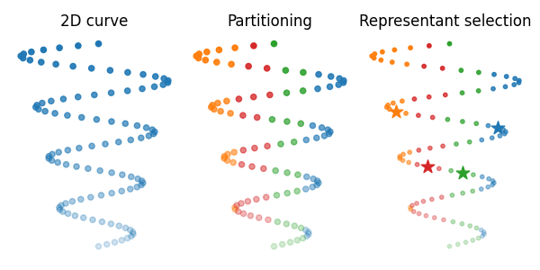
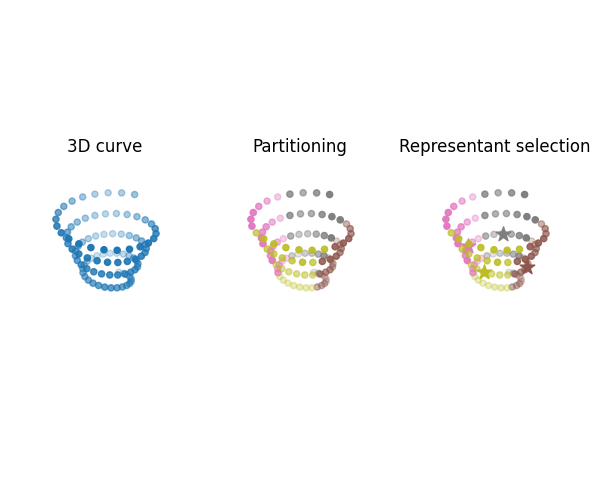
Visualize partitioned attributed point clouds

Compute the partitioning and representant selection further used within qFGW wrapper, both provided by a K-means algorithm. Then visualize partitioned spaces.

part1, rep_indices1 = get_partition_and_representants_samples(
    X, 4, 'kmeans', 0)
part2, rep_indices2 = get_partition_and_representants_samples(
    Y, 4, 'kmeans', 0)

upart1 = np.unique(part1)
upart2 = np.unique(part2)

# Plot the source and target samples as distributions
s = 20
fig = plt.figure(3, figsize=(6, 3))

ax1 = fig.add_subplot(1, 3, 1)
ax1.set_title("2D curve")
ax1.scatter(X[:, 0], X[:, 1], color="C0", alpha=FX, s=s)
plt.axis('off')


ax2 = fig.add_subplot(1, 3, 2)
ax2.set_title("Partitioning")
for i, elem in enumerate(upart1):
    idx = np.argwhere(part1 == elem)[:, 0]
    ax2.scatter(X[idx, 0], X[idx, 1], color="C%s" % i, alpha=FX[idx], s=s)
plt.axis('off')

ax3 = fig.add_subplot(1, 3, 3)
ax3.set_title("Representant selection")
for i, elem in enumerate(upart1):
    idx = np.argwhere(part1 == elem)[:, 0]
    ax3.scatter(X[idx, 0], X[idx, 1], color="C%s" % i, alpha=FX[idx], s=10)
    rep_idx = rep_indices1[i]
    ax3.scatter([X[rep_idx, 0]], [X[rep_idx, 1]], color="C%s" % i, alpha=1, s=6 * s, marker='*')
plt.axis('off')
plt.tight_layout()
plt.show()

start_color = upart1.shape[0] + 1

fig = plt.figure(4, figsize=(6, 5))

ax4 = fig.add_subplot(1, 3, 1, projection="3d")
ax4.set_title("3D curve")
ax4.scatter(Y[:, 0], Y[:, 1], Y[:, 2], c='C0', alpha=FY, s=s)
plt.axis('off')

ax5 = fig.add_subplot(1, 3, 2, projection="3d")
ax5.set_title("Partitioning")
for i, elem in enumerate(upart2):
    idx = np.argwhere(part2 == elem)[:, 0]
    color = 'C%s' % (start_color + i)
    ax5.scatter(Y[idx, 0], Y[idx, 1], Y[idx, 2], c=color, alpha=FY[idx], s=s)
plt.axis('off')

ax6 = fig.add_subplot(1, 3, 3, projection="3d")
ax6.set_title("Representant selection")
for i, elem in enumerate(upart2):
    idx = np.argwhere(part2 == elem)[:, 0]
    color = 'C%s' % (start_color + i)
    rep_idx = rep_indices2[i]
    ax6.scatter(Y[idx, 0], Y[idx, 1], Y[idx, 2], c=color, alpha=FY[idx], s=s)
    ax6.scatter([Y[rep_idx, 0]], [Y[rep_idx, 1]], [Y[rep_idx, 2]], c=color, alpha=1, s=6 * s, marker='*')
plt.axis('off')
plt.tight_layout()
plt.show()

• 
• 

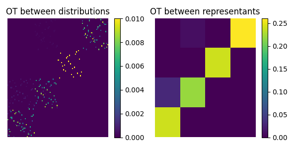
Compute the quantized Fused Gromov-Wasserstein distance between samples using the wrapper

Compute qFGW(X, FX, hX, Y, FY, HY), setting the trade-off parameter between structures and features alpha=0.5. This solver considers a squared euclidean structure for each distribution X and Y, and partition each of them into 4 clusters using the K-means algorithm before computing qFGW.

T_global, Ts_local, T, log = quantized_fused_gromov_wasserstein_samples(
    X, Y, 4, 4, p=None, q=None, F1=FX[:, None], F2=FY[:, None], alpha=0.5,
    method='kmeans', log=True)

# Plot low rank GW with different ranks
pl.figure(5, figsize=(6, 3))
pl.subplot(1, 2, 1)
pl.title('OT between distributions')
pl.imshow(T, interpolation="nearest", aspect="auto")
pl.colorbar()
pl.axis('off')

pl.subplot(1, 2, 2)
pl.title('OT between representants')
pl.imshow(T_global, interpolation="nearest", aspect="auto")
pl.axis('off')
pl.colorbar()

pl.tight_layout()
pl.show()