Graph classification with Tempate Based Fused Gromov Wasserstein

This example first illustrates how to train a graph classification gnn based on the Template Fused Gromov Wasserstein layer as proposed in [52] .

[53] C. Vincent-Cuaz, R. Flamary, M. Corneli, T. Vayer, N. Courty (2022).Template based graph neural network with optimal transport distances. Advances in Neural Information Processing Systems, 35.

# Author: Sonia Mazelet <sonia.mazelet@ens-paris-saclay.fr>
#         Rémi Flamary <remi.flamary@unice.fr>
#
# License: MIT License

# sphinx_gallery_thumbnail_number = 1

import matplotlib.pyplot as pl
import torch
import networkx as nx
from torch.utils.data import random_split
from torch_geometric.loader import DataLoader
from torch_geometric.utils import to_networkx, one_hot
from torch_geometric.utils import stochastic_blockmodel_graph as sbm
from torch_geometric.data import Data as GraphData
import torch.nn as nn
from torch_geometric.nn import Linear, GCNConv
from ot.gnn import TFGWPooling
from sklearn.manifold import TSNE

Generate data

# parameters

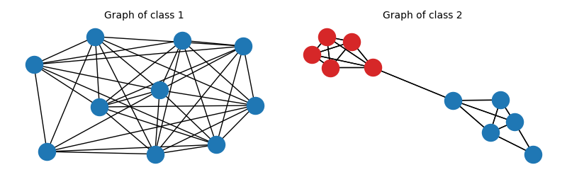
# We create 2 classes of stochastic block models (SBM) graphs with 1 block and 2 blocks respectively.

torch.manual_seed(0)

n_graphs = 50
n_nodes = 10
n_node_classes = 2

#edge probabilities for the SBMs
P1 = [[0.8]]
P2 = [[0.9, 0.1], [0.1, 0.9]]

#block sizes
block_sizes1 = [n_nodes]
block_sizes2 = [n_nodes // 2, n_nodes // 2]

#node features
x1 = torch.tensor([0, 0, 0, 0, 0, 0, 0, 0, 0, 0])
x1 = one_hot(x1, num_classes=n_node_classes)
x1 = torch.reshape(x1, (n_nodes, n_node_classes))

x2 = torch.tensor([0, 0, 0, 0, 0, 1, 1, 1, 1, 1])
x2 = one_hot(x2, num_classes=n_node_classes)
x2 = torch.reshape(x2, (n_nodes, n_node_classes))

graphs1 = [GraphData(x=x1, edge_index=sbm(block_sizes1, P1), y=torch.tensor([0])) for i in range(n_graphs)]
graphs2 = [GraphData(x=x2, edge_index=sbm(block_sizes2, P2), y=torch.tensor([1])) for i in range(n_graphs)]

graphs = graphs1 + graphs2

#split the data into train and test sets
train_graphs, test_graphs = random_split(graphs, [n_graphs, n_graphs])

train_loader = DataLoader(train_graphs, batch_size=10, shuffle=True)
test_loader = DataLoader(test_graphs, batch_size=10, shuffle=False)

Plot data

# plot one graph of each class

fontsize = 10

pl.figure(0, figsize=(8, 2.5))
pl.clf()
pl.subplot(121)
pl.axis('off')
pl.title('Graph of class 1', fontsize=fontsize)
G = to_networkx(graphs1[0], to_undirected=True)
pos = nx.spring_layout(G, seed=0)
nx.draw_networkx(G, pos, with_labels=False, node_color="tab:blue")

pl.subplot(122)
pl.axis('off')
pl.title('Graph of class 2', fontsize=fontsize)
G = to_networkx(graphs2[0], to_undirected=True)
pos = nx.spring_layout(G, seed=0)
nx.draw_networkx(G, pos, with_labels=False, nodelist=[0, 1, 2, 3, 4], node_color="tab:blue")
nx.draw_networkx(G, pos, with_labels=False, nodelist=[5, 6, 7, 8, 9], node_color="tab:red")

pl.tight_layout()
pl.show()

Pooling architecture using the TFGW layer

class pooling_TFGW(nn.Module):
    """
    Pooling architecture using the TFGW layer.
    """

    def __init__(self, n_features, n_templates, n_template_nodes, n_classes, n_hidden_layers, feature_init_mean=0., feature_init_std=1.):
        """
        Pooling architecture using the TFGW layer.
        """
        super().__init__()

        self.n_templates = n_templates
        self.n_template_nodes = n_template_nodes
        self.n_hidden_layers = n_hidden_layers
        self.n_features = n_features

        self.conv = GCNConv(self.n_features, self.n_hidden_layers)

        self.TFGW = TFGWPooling(self.n_hidden_layers, self.n_templates, self.n_template_nodes, feature_init_mean=feature_init_mean, feature_init_std=feature_init_std)

        self.linear = Linear(self.n_templates, n_classes)

    def forward(self, x, edge_index, batch=None):
        x = self.conv(x, edge_index)

        x = self.TFGW(x, edge_index, batch)

        x_latent = x  # save latent embeddings for visualization

        x = self.linear(x)

        return x, x_latent

Graph classification training

n_epochs = 25

#store latent embeddings and classes for TSNE visualization
embeddings_for_TSNE = []
classes = []

model = pooling_TFGW(n_features=2, n_templates=2, n_template_nodes=2, n_classes=2, n_hidden_layers=2, feature_init_mean=0.5, feature_init_std=0.5)

optimizer = torch.optim.Adam(model.parameters(), lr=0.005, weight_decay=0.0005)
criterion = torch.nn.CrossEntropyLoss()

all_accuracy = []
all_loss = []

for epoch in range(n_epochs):

    losses = []
    accs = []

    for data in train_loader:
        out, latent_embedding = model(data.x, data.edge_index, data.batch)
        loss = criterion(out, data.y)
        loss.backward()
        optimizer.step()

        pred = out.argmax(dim=1)
        train_correct = pred == data.y
        train_acc = int(train_correct.sum()) / len(data)

        accs.append(train_acc)
        losses.append(loss.item())

        #store last classes and embeddings for TSNE visualization
        if epoch == n_epochs - 1:
            embeddings_for_TSNE.append(latent_embedding)
            classes.append(data.y)

    print(f'Epoch: {epoch:03d}, Loss: {torch.mean(torch.tensor(losses)):.4f},Train Accuracy: {torch.mean(torch.tensor(accs)):.4f}')

    all_accuracy.append(torch.mean(torch.tensor(accs)))
    all_loss.append(torch.mean(torch.tensor(losses)))


pl.figure(1, figsize=(8, 2.5))
pl.clf()
pl.subplot(121)
pl.plot(all_loss)
pl.xlabel('epochs')
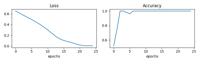
pl.title('Loss')

pl.subplot(122)
pl.plot(all_accuracy)
pl.xlabel('epochs')
pl.title('Accuracy')

pl.tight_layout()
pl.show()

#Test

test_accs = []

for data in test_loader:
    out, latent_embedding = model(data.x, data.edge_index, data.batch)
    pred = out.argmax(dim=1)
    test_correct = pred == data.y
    test_acc = int(test_correct.sum()) / len(data)
    test_accs.append(test_acc)
    embeddings_for_TSNE.append(latent_embedding)
    classes.append(data.y)

classes = torch.hstack(classes)

print(f'Test Accuracy: {torch.mean(torch.tensor(test_acc)):.4f}')

Epoch: 000, Loss: 0.6519,Train Accuracy: 0.5200
Epoch: 001, Loss: 0.6222,Train Accuracy: 0.7400
Epoch: 002, Loss: 0.5858,Train Accuracy: 1.0000
Epoch: 003, Loss: 0.5570,Train Accuracy: 1.0000
Epoch: 004, Loss: 0.5235,Train Accuracy: 0.9800
Epoch: 005, Loss: 0.4945,Train Accuracy: 0.9600
Epoch: 006, Loss: 0.4596,Train Accuracy: 1.0000
Epoch: 007, Loss: 0.4248,Train Accuracy: 1.0000
Epoch: 008, Loss: 0.3868,Train Accuracy: 1.0000
Epoch: 009, Loss: 0.3455,Train Accuracy: 1.0000
Epoch: 010, Loss: 0.3008,Train Accuracy: 1.0000
Epoch: 011, Loss: 0.2525,Train Accuracy: 1.0000
Epoch: 012, Loss: 0.2050,Train Accuracy: 1.0000
Epoch: 013, Loss: 0.1598,Train Accuracy: 1.0000
Epoch: 014, Loss: 0.1277,Train Accuracy: 1.0000
Epoch: 015, Loss: 0.1046,Train Accuracy: 1.0000
Epoch: 016, Loss: 0.0875,Train Accuracy: 1.0000
Epoch: 017, Loss: 0.0725,Train Accuracy: 1.0000
Epoch: 018, Loss: 0.0554,Train Accuracy: 1.0000
Epoch: 019, Loss: 0.0355,Train Accuracy: 1.0000
Epoch: 020, Loss: 0.0194,Train Accuracy: 1.0000
Epoch: 021, Loss: 0.0095,Train Accuracy: 1.0000
Epoch: 022, Loss: 0.0052,Train Accuracy: 1.0000
Epoch: 023, Loss: 0.0047,Train Accuracy: 1.0000
Epoch: 024, Loss: 0.0054,Train Accuracy: 1.0000
Test Accuracy: 1.0000

indices = torch.randint(2 * n_graphs, (60,))  # select a subset of embeddings for TSNE visualization
latent_embeddings = torch.vstack(embeddings_for_TSNE).detach().numpy()[indices, :]

TSNE_embeddings = TSNE(n_components=2, perplexity=20, random_state=1).fit_transform(latent_embeddings)

class_0 = classes[indices] == 0
class_1 = classes[indices] == 1

TSNE_embeddings_0 = TSNE_embeddings[class_0, :]
TSNE_embeddings_1 = TSNE_embeddings[class_1, :]

pl.figure(2, figsize=(6, 2.5))
pl.scatter(TSNE_embeddings_0[:, 0], TSNE_embeddings_0[:, 1],
           alpha=0.5, marker='o', label='class 1')
pl.scatter(TSNE_embeddings_1[:, 0], TSNE_embeddings_1[:, 1],
           alpha=0.5, marker='o', label='class 2')
pl.legend()
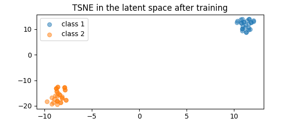
pl.title('TSNE in the latent space after training')
pl.show()