Note
Go to the end to download the full example code.
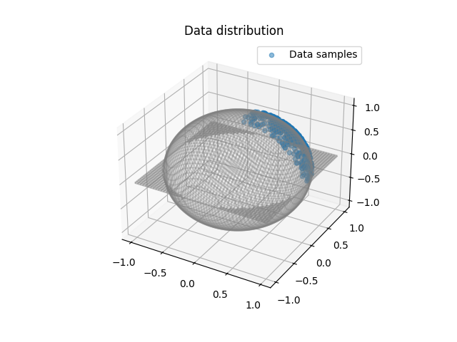
Spherical Sliced-Wasserstein Embedding on Sphere
Here, we aim at transforming samples into a uniform distribution on the sphere by minimizing SSW:
\[\min_{x} SSW_2(\nu, \frac{1}{n}\sum_{i=1}^n \delta_{x_i})\]
where \(\nu=\mathrm{Unif}(S^{d-1})\).
# Author: Clément Bonet <clement.bonet@univ-ubs.fr>
#
# License: MIT License

# sphinx_gallery_thumbnail_number = 3

import numpy as np
import matplotlib.pyplot as pl
import matplotlib.animation as animation
import torch
import torch.nn.functional as F

import ot
Data generation
torch.manual_seed(1)

N = 500
x0 = torch.rand(N, 3)
x0 = F.normalize(x0, dim=-1)
Plot data
def plot_sphere(ax):
    # Create a sphere using spherical coordinates
    phi = np.linspace(0, 2 * np.pi, 100)
    theta = np.linspace(0, np.pi, 100)
    phi, theta = np.meshgrid(phi, theta)

    # Compute the spherical coordinates
    X = np.sin(theta) * np.cos(phi)
    Y = np.sin(theta) * np.sin(phi)
    Z = np.cos(theta)

    # Plot the wireframe
    ax.plot_wireframe(X, Y, Z, color="gray", alpha=0.3)


# plot the distributions
pl.figure(1)
ax = pl.axes(projection="3d")
plot_sphere(ax)
ax.scatter(x0[:, 0], x0[:, 1], x0[:, 2], label="Data samples", alpha=0.5)
ax.set_title("Data distribution")
ax.legend()
<matplotlib.legend.Legend object at 0x7e97aa920bf0>
Gradient descent
x = x0.clone()
x.requires_grad_(True)

n_iter = 100
lr = 150

losses = []
xvisu = torch.zeros(n_iter, N, 3)

for i in range(n_iter):
    sw = ot.sliced_wasserstein_sphere_unif(x, n_projections=500)
    grad_x = torch.autograd.grad(sw, x)[0]

    x = x - lr * grad_x / np.sqrt(i / 10 + 1)
    x = F.normalize(x, p=2, dim=1)

    losses.append(sw.item())
    xvisu[i, :, :] = x.detach().clone()

    if i % 100 == 0:
        print("Iter: {:3d}, loss={}".format(i, losses[-1]))

pl.figure(1)
pl.semilogy(losses)
pl.grid()
pl.title("SSW")
pl.xlabel("Iterations")
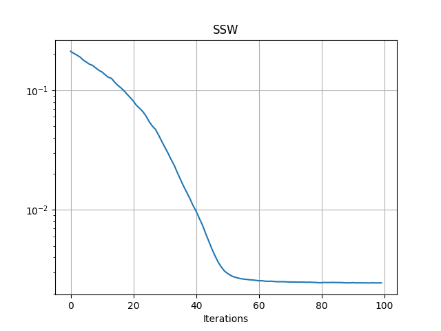
Iter:   0, loss=0.21037161350250244

Text(0.5, 23.633333333333333, 'Iterations')
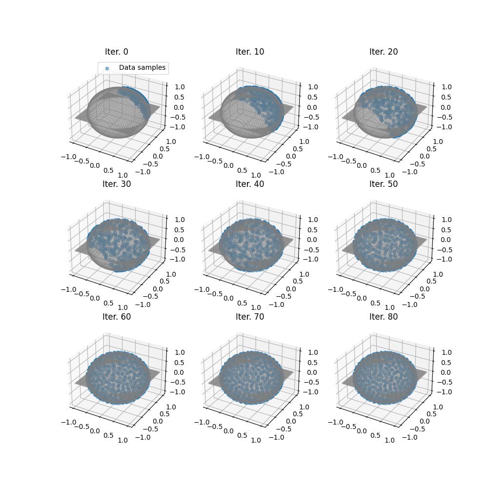
Plot trajectories of generated samples along iterations
ivisu = [0, 10, 20, 30, 40, 50, 60, 70, 80]

fig = pl.figure(3, (10, 10))
for i in range(9):
    # pl.subplot(3, 3, i + 1)
    # ax = pl.axes(projection='3d')
    ax = fig.add_subplot(3, 3, i + 1, projection="3d")
    plot_sphere(ax)
    ax.scatter(
        xvisu[ivisu[i], :, 0],
        xvisu[ivisu[i], :, 1],
        xvisu[ivisu[i], :, 2],
        label="Data samples",
        alpha=0.5,
    )
    ax.set_title("Iter. {}".format(ivisu[i]))
    # ax.axis("off")
    if i == 0:
        ax.legend()
Animate trajectories of generated samples along iteration
pl.figure(4, (8, 8))


def _update_plot(i):
    i = 3 * i
    pl.clf()
    ax = pl.axes(projection="3d")
    plot_sphere(ax)
    ax.scatter(
        xvisu[i, :, 0], xvisu[i, :, 1], xvisu[i, :, 2], label="Data samples$", alpha=0.5
    )
    ax.axis("off")
    ax.set_xlim((-1.5, 1.5))
    ax.set_ylim((-1.5, 1.5))
    ax.set_title("Iter. {}".format(i))
    return 1


print(xvisu.shape)

i = 0
ax = pl.axes(projection="3d")
plot_sphere(ax)
ax.scatter(
    xvisu[i, :, 0],
    xvisu[i, :, 1],
    xvisu[i, :, 2],
    label="Data samples from $G\#\mu_n$",
    alpha=0.5,
)
ax.axis("off")
ax.set_xlim((-1.5, 1.5))
ax.set_ylim((-1.5, 1.5))
ax.set_title("Iter. {}".format(ivisu[i]))


ani = animation.FuncAnimation(
    pl.gcf(), _update_plot, n_iter // 5, interval=200, repeat_delay=2000
)
/home/circleci/project/examples/backends/plot_ssw_unif_torch.py:161: SyntaxWarning: invalid escape sequence '\#'
  label="Data samples from $G\#\mu_n$",
torch.Size([100, 500, 3])
Total running time of the script: (0 minutes 12.574 seconds)