2D free support Sinkhorn barycenters of distributions

Illustration of Sinkhorn barycenter calculation between empirical distributions understood as point clouds

# Authors: Eduardo Fernandes Montesuma <eduardo.fernandes-montesuma@universite-paris-saclay.fr>
#
# License: MIT License

import numpy as np
import matplotlib.pyplot as plt
import ot

General Parameters

reg = 1e-2  # Entropic Regularization
numItermax = 20  # Maximum number of iterations for the Barycenter algorithm
numInnerItermax = 50  # Maximum number of sinkhorn iterations
n_samples = 200

Generate Data

X1 = np.random.randn(200, 2)
X2 = 2 * np.concatenate(
    [
        np.concatenate([-np.ones([50, 1]), np.linspace(-1, 1, 50)[:, None]], axis=1),
        np.concatenate([np.linspace(-1, 1, 50)[:, None], np.ones([50, 1])], axis=1),
        np.concatenate([np.ones([50, 1]), np.linspace(1, -1, 50)[:, None]], axis=1),
        np.concatenate([np.linspace(1, -1, 50)[:, None], -np.ones([50, 1])], axis=1),
    ],
    axis=0,
)
X3 = np.random.randn(200, 2)
X3 = 2 * (X3 / np.linalg.norm(X3, axis=1)[:, None])
X4 = np.random.multivariate_normal(
    np.array([0, 0]), np.array([[1.0, 0.5], [0.5, 1.0]]), size=200
)

a1, a2, a3, a4 = ot.unif(len(X1)), ot.unif(len(X1)), ot.unif(len(X1)), ot.unif(len(X1))

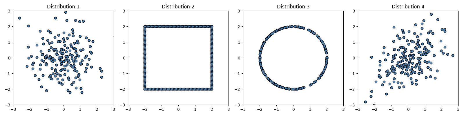
Inspect generated distributions

fig, axes = plt.subplots(1, 4, figsize=(16, 4))

axes[0].scatter(x=X1[:, 0], y=X1[:, 1], c="steelblue", edgecolor="k")
axes[1].scatter(x=X2[:, 0], y=X2[:, 1], c="steelblue", edgecolor="k")
axes[2].scatter(x=X3[:, 0], y=X3[:, 1], c="steelblue", edgecolor="k")
axes[3].scatter(x=X4[:, 0], y=X4[:, 1], c="steelblue", edgecolor="k")

axes[0].set_xlim([-3, 3])
axes[0].set_ylim([-3, 3])
axes[0].set_title("Distribution 1")

axes[1].set_xlim([-3, 3])
axes[1].set_ylim([-3, 3])
axes[1].set_title("Distribution 2")

axes[2].set_xlim([-3, 3])
axes[2].set_ylim([-3, 3])
axes[2].set_title("Distribution 3")

axes[3].set_xlim([-3, 3])
axes[3].set_ylim([-3, 3])
axes[3].set_title("Distribution 4")

plt.tight_layout()
plt.show()

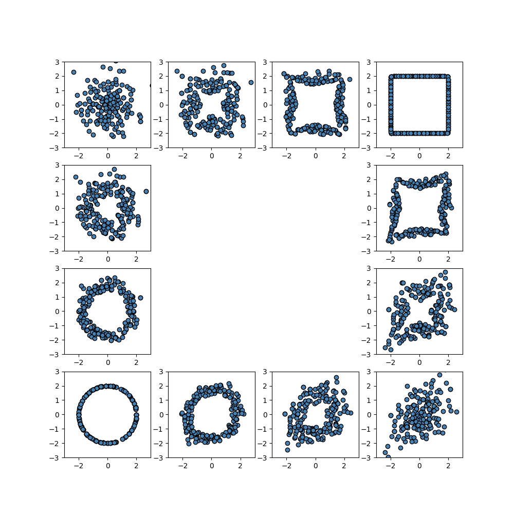
Interpolating Empirical Distributions

fig = plt.figure(figsize=(10, 10))

weights = np.array(
    [
        [3 / 3, 0 / 3],
        [2 / 3, 1 / 3],
        [1 / 3, 2 / 3],
        [0 / 3, 3 / 3],
    ]
).astype(np.float32)

for k in range(4):
    XB_init = np.random.randn(n_samples, 2)
    XB = ot.bregman.free_support_sinkhorn_barycenter(
        measures_locations=[X1, X2],
        measures_weights=[a1, a2],
        weights=weights[k],
        X_init=XB_init,
        reg=reg,
        numItermax=numItermax,
        numInnerItermax=numInnerItermax,
    )
    ax = plt.subplot2grid((4, 4), (0, k))
    ax.scatter(XB[:, 0], XB[:, 1], color="steelblue", edgecolor="k")
    ax.set_xlim([-3, 3])
    ax.set_ylim([-3, 3])

for k in range(1, 4, 1):
    XB_init = np.random.randn(n_samples, 2)
    XB = ot.bregman.free_support_sinkhorn_barycenter(
        measures_locations=[X1, X3],
        measures_weights=[a1, a2],
        weights=weights[k],
        X_init=XB_init,
        reg=reg,
        numItermax=numItermax,
        numInnerItermax=numInnerItermax,
    )
    ax = plt.subplot2grid((4, 4), (k, 0))
    ax.scatter(XB[:, 0], XB[:, 1], color="steelblue", edgecolor="k")
    ax.set_xlim([-3, 3])
    ax.set_ylim([-3, 3])

for k in range(1, 4, 1):
    XB_init = np.random.randn(n_samples, 2)
    XB = ot.bregman.free_support_sinkhorn_barycenter(
        measures_locations=[X3, X4],
        measures_weights=[a1, a2],
        weights=weights[k],
        X_init=XB_init,
        reg=reg,
        numItermax=numItermax,
        numInnerItermax=numInnerItermax,
    )
    ax = plt.subplot2grid((4, 4), (3, k))
    ax.scatter(XB[:, 0], XB[:, 1], color="steelblue", edgecolor="k")
    ax.set_xlim([-3, 3])
    ax.set_ylim([-3, 3])

for k in range(1, 3, 1):
    XB_init = np.random.randn(n_samples, 2)
    XB = ot.bregman.free_support_sinkhorn_barycenter(
        measures_locations=[X2, X4],
        measures_weights=[a1, a2],
        weights=weights[k],
        X_init=XB_init,
        reg=reg,
        numItermax=numItermax,
        numInnerItermax=numInnerItermax,
    )
    ax = plt.subplot2grid((4, 4), (k, 3))
    ax.scatter(XB[:, 0], XB[:, 1], color="steelblue", edgecolor="k")
    ax.set_xlim([-3, 3])
    ax.set_ylim([-3, 3])

plt.show()

/home/circleci/project/ot/bregman/_sinkhorn.py:667: UserWarning: Sinkhorn did not converge. You might want to increase the number of iterations `numItermax` or the regularization parameter `reg`.
  warnings.warn(