Numerically-stable entropic partial Wasserstein (log-domain solver)

Note

Example added in release: 0.9.7.

ot.partial.entropic_partial_wasserstein is numerically unstable at small regularisation: the iterates underflow to zero and the returned plan contains NaNs (see PythonOT/POT issue #723). This example reproduces the failure mode on a small problem and shows that the log-domain solver, selected with entropic_partial_wasserstein(..., method='sinkhorn_log') (equivalently ot.partial.entropic_partial_wasserstein_logscale), produces a finite plan over the same sweep, agreeing with the original solver at large reg and degrading gracefully at small reg.

Following the ot.sinkhorn convention, the solver to use is chosen through the method parameter: 'sinkhorn' (default) for the classical solver and 'sinkhorn_log' for the log-domain one. The log-domain solver is slower per iteration than the standard one, so the recommendation is to use the standard solver by default and fall back to the log-domain solver when reg is small enough to risk underflow.

# Author: wzm2256 <wzm2256@qq.com> (original PR #724)
# License: MIT License

import numpy as np
import scipy as sp
import matplotlib.pylab as pl

import ot

Construct a 50x50 cost matrix

Mirrors the cost-matrix scale (~50) used in PythonOT/POT issue #723.

rng = np.random.RandomState(0)
n = 50
xs = rng.rand(n, 2)
xt = rng.rand(n, 2)
M = sp.spatial.distance.cdist(xs, xt) * 50.0

a = np.ones(n) / n
b = np.ones(n) / n
m = 0.6  # transport ~60% of the mass

Sweep regularisation

Run both solvers across a range of reg values. On this 50×50 problem at cost-scale 50 the standard solver returns NaN at the reg values closest to the underflow boundary (typically reg ~0.05–0.01 in our runs, though the exact transition depends on the BLAS / platform’s float64 underflow behaviour); the log-domain solver stays finite over the whole sweep, including the very small reg regime where the standard exp(−M/reg) path would underflow to zero everywhere.

regs = [1.0, 0.5, 0.1, 0.05, 0.01, 5e-3, 1e-3, 5e-4]
standard_finite = []
logscale_finite = []
standard_mass = []
logscale_mass = []

for reg in regs:
    G_std = ot.partial.entropic_partial_wasserstein(
        a, b, M, reg=reg, m=m, numItermax=2000
    )
    G_log = ot.partial.entropic_partial_wasserstein(
        a, b, M, reg=reg, m=m, method="sinkhorn_log", numItermax=2000
    )
    standard_finite.append(bool(np.isfinite(G_std).all()))
    logscale_finite.append(bool(np.isfinite(G_log).all()))
    standard_mass.append(float(G_std.sum()) if np.isfinite(G_std).all() else np.nan)
    logscale_mass.append(float(G_log.sum()))

print(
    "reg          standard_finite logscale_finite  std_mass logscale_mass (target m={:.2f})".format(
        m
    )
)
for reg, sf, lf, sm, lm in zip(
    regs, standard_finite, logscale_finite, standard_mass, logscale_mass
):
    print(f"{reg:>10.4g}   {str(sf):<14}  {str(lf):<14}  {sm:>8.3f}      {lm:>8.3f}")

/home/circleci/project/ot/partial/partial_solvers.py:620: RuntimeWarning: invalid value encountered in divide
  q1 = q1 * Kprev / K1
/home/circleci/project/ot/partial/partial_solvers.py:624: RuntimeWarning: invalid value encountered in divide
  q2 = q2 * K1prev / K2
/home/circleci/project/ot/partial/partial_solvers.py:628: RuntimeWarning: invalid value encountered in divide
  q3 = q3 * K2prev / K
Warning: numerical errors at iteration 1
/home/circleci/project/ot/partial/partial_solvers.py:619: RuntimeWarning: divide by zero encountered in divide
  K1 = nx.dot(nx.diag(nx.minimum(a / nx.sum(K, axis=1), dx)), K)
/home/circleci/project/ot/partial/partial_solvers.py:619: RuntimeWarning: overflow encountered in divide
  K1 = nx.dot(nx.diag(nx.minimum(a / nx.sum(K, axis=1), dx)), K)
/home/circleci/project/ot/partial/partial_solvers.py:623: RuntimeWarning: divide by zero encountered in divide
  K2 = nx.dot(K1, nx.diag(nx.minimum(b / nx.sum(K1, axis=0), dy)))
Warning: numerical errors at iteration 1
reg          standard_finite logscale_finite  std_mass logscale_mass (target m=0.60)
         1   True            True               0.600         0.600
       0.5   True            True               0.600         0.600
       0.1   True            True               0.600         0.600
      0.05   False           True                 nan         0.600
      0.01   False           True                 nan         0.600
     0.005   True            True               0.600         0.600
     0.001   True            True               0.600         0.600
    0.0005   True            True               0.600         0.600

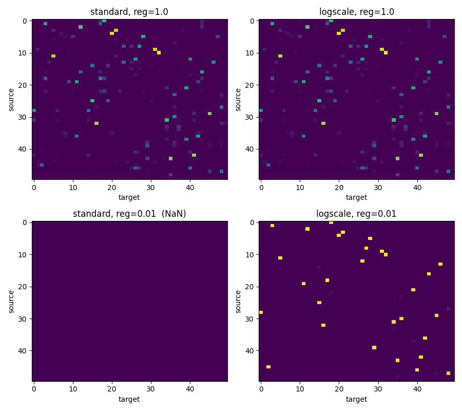
Plot the resulting plans at large vs. small reg

fig, axes = pl.subplots(2, 2, figsize=(9, 8))
for ax, reg in zip(axes[:, 0], (1.0, 0.01)):
    G_std = ot.partial.entropic_partial_wasserstein(
        a, b, M, reg=reg, m=m, numItermax=2000
    )
    if not np.isfinite(G_std).all():
        G_std = np.zeros_like(G_std)
        ax.set_title(f"standard, reg={reg}  (NaN)")
    else:
        ax.set_title(f"standard, reg={reg}")
    ax.imshow(G_std, cmap="viridis", aspect="auto")
    ax.set_xlabel("target")
    ax.set_ylabel("source")

for ax, reg in zip(axes[:, 1], (1.0, 0.01)):
    G_log = ot.partial.entropic_partial_wasserstein(
        a, b, M, reg=reg, m=m, method="sinkhorn_log", numItermax=2000
    )
    ax.set_title(f"logscale, reg={reg}")
    ax.imshow(G_log, cmap="viridis", aspect="auto")
    ax.set_xlabel("target")
    ax.set_ylabel("source")

fig.tight_layout()
pl.show()

Warning: numerical errors at iteration 1