Note
Go to the end to download the full example code.
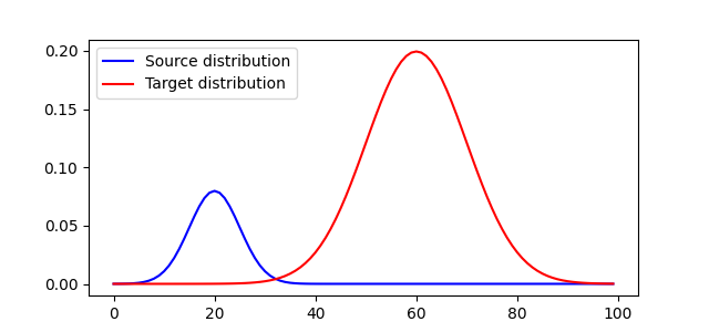
1D Unbalanced optimal transport
This example illustrates the computation of Unbalanced Optimal transport using a Kullback-Leibler relaxation.
# Author: Hicham Janati <hicham.janati@inria.fr>
#         Clément Bonet <clement.bonet.mapp@polytechnique.edu>
#
# License: MIT License

# sphinx_gallery_thumbnail_number = 4

import numpy as np
import matplotlib.pylab as pl
import ot
import ot.plot
from ot.datasets import make_1D_gauss as gauss
import torch
Generate data
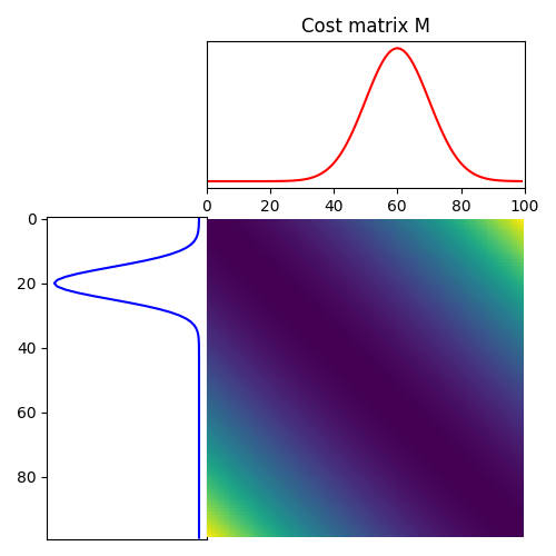
Plot distributions and loss matrix
(<Axes: >, <Axes: >, <Axes: >)
Solve Unbalanced OT with MM Unbalanced
alpha = 1.0 # Unbalanced KL relaxation parameter
Gs, log = ot.unbalanced.mm_unbalanced(a, b, M / M.max(), alpha, verbose=False, log=True)
pl.figure(3, figsize=(5, 5))
ot.plot.plot1D_mat(a, b, Gs, "UOT plan")
pl.show()
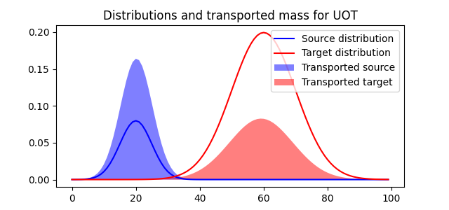
pl.figure(4, figsize=(6.4, 3))
pl.plot(x, a, "b", label="Source distribution")
pl.plot(x, b, "r", label="Target distribution")
pl.fill(x, Gs.sum(1), "b", alpha=0.5, label="Transported source")
pl.fill(x, Gs.sum(0), "r", alpha=0.5, label="Transported target")
pl.legend(loc="upper right")
pl.title("Distributions and transported mass for UOT")
pl.show()
print("Mass of reweighted marginals:", Gs.sum())
print("Unbalanced OT loss:", log["total_cost"] * M.max())
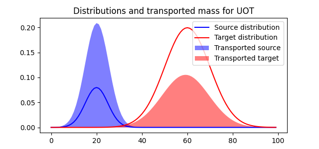
Mass of reweighted marginals: 2.061425461509171
Unbalanced OT loss: 18397.928984107042
Solve 1D UOT with Frank-Wolfe
alpha = M.max() # Unbalanced KL relaxation parameter
a_reweighted, b_reweighted, loss = ot.unbalanced.uot_1d(
torch.tensor(x, dtype=torch.float64),
torch.tensor(x, dtype=torch.float64),
alpha,
u_weights=torch.tensor(a, dtype=torch.float64),
v_weights=torch.tensor(b, dtype=torch.float64),
p=2,
returnCost="total",
)
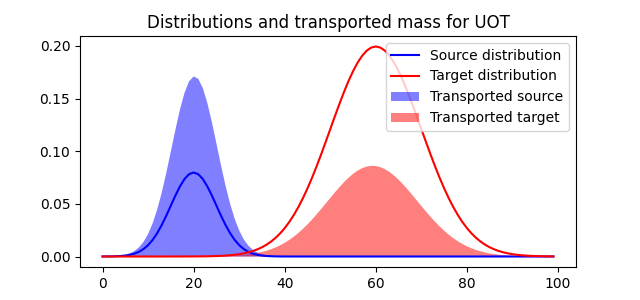
pl.figure(4, figsize=(6.4, 3))
pl.plot(x, a, "b", label="Source distribution")
pl.plot(x, b, "r", label="Target distribution")
pl.fill(x, a_reweighted, "b", alpha=0.5, label="Transported source")
pl.fill(x, b_reweighted, "r", alpha=0.5, label="Transported target")
pl.legend(loc="upper right")
pl.title("Distributions and transported mass for UOT")
pl.show()
print("Mass of reweighted marginals:", a_reweighted.sum().item())
print("Unbalanced OT loss:", loss.item())
Mass of reweighted marginals: 2.062383712135279
Unbalanced OT loss: 18379.180712239286
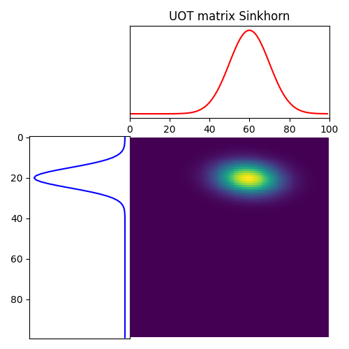
Solve Unbalanced Sinkhorn
# Sinkhorn
epsilon = 0.1 # entropy parameter
alpha = 1.0 # Unbalanced KL relaxation parameter
Gs = ot.unbalanced.sinkhorn_unbalanced(a, b, M / M.max(), epsilon, alpha, verbose=True)
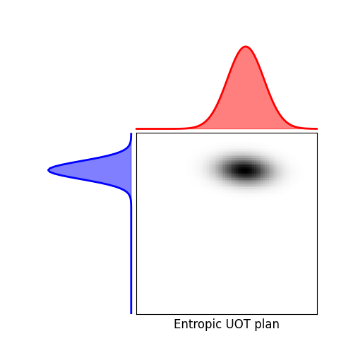
pl.figure(3, figsize=(5, 5))
ot.plot.plot1D_mat(a, b, Gs, "Entropic UOT plan")
pl.show()
pl.figure(4, figsize=(6.4, 3))
pl.plot(x, a, "b", label="Source distribution")
pl.plot(x, b, "r", label="Target distribution")
pl.fill(x, Gs.sum(1), "b", alpha=0.5, label="Transported source")
pl.fill(x, Gs.sum(0), "r", alpha=0.5, label="Transported target")
pl.legend(loc="upper right")
pl.title("Distributions and transported mass for UOT")
pl.show()
print("Mass of reweighted marginals:", Gs.sum())
Mass of reweighted marginals: 2.1410336580797993
Total running time of the script: (0 minutes 0.613 seconds)