Sliced Unbalanced optimal transport

This example illustrates the behavior of Sliced UOT versus Unbalanced Sliced OT, introduced in [82]. The first one removes outliers on each slice while the second one removes outliers of the original marginals.

[82] Bonet, C., Nadjahi, K., Séjourné, T., Fatras, K., & Courty, N. (2025). Slicing Unbalanced Optimal Transport. Transactions on Machine Learning Research.

# Author: Clément Bonet <clement.bonet.mapp@polytechnique.edu>
#         Nicolas Courty <nicolas.courty@irisa.fr>
#
# License: MIT License

# sphinx_gallery_thumbnail_number = 4

import numpy as np
import matplotlib.pylab as pl
import ot
import torch
import matplotlib.pyplot as plt
import matplotlib.animation as animation

from sklearn.neighbors import KernelDensity

Generate data

np.random.seed(42)

n_samples = 25  # 500
nb_outliers = 10  # 200


mu_s = np.array([0, 0]) - 0.5
cov_s = 0.2**2 * np.array([[1, 0], [0, 1]])

mu_s_outliers = -np.array([2, 0.5])
cov_s_outliers = 0.05**2 * np.array([[1, 0], [0, 1]])

mu_t = np.array([0, 0]) + 1.5
cov_t = 0.2**2 * np.array([[1, 0], [0, 1]])


def generate_dataset(n_samples):
    # Generate source data (with outliers)
    Xs = ot.datasets.make_2D_samples_gauss(n_samples, mu_s, cov_s)
    Xs_outlier = ot.datasets.make_2D_samples_gauss(
        nb_outliers, mu_s_outliers, cov_s_outliers
    )

    Xs = np.vstack((Xs, Xs_outlier))
    Xs_torch = torch.from_numpy(Xs).type(torch.float)

    # Generate target data
    Xt = ot.datasets.make_2D_samples_gauss(n_samples, mu_t, cov_t)
    Xt_torch = torch.from_numpy(Xt).type(torch.float)

    return Xs_torch, Xt_torch


Xs, Xt = generate_dataset(n_samples)

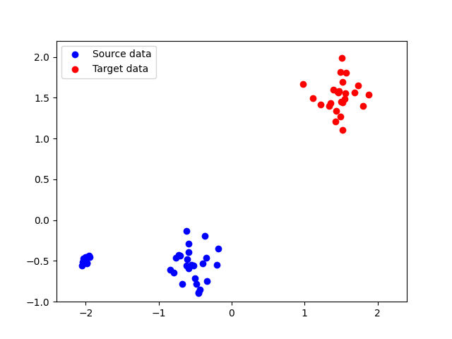
pl.figure(1)
pl.scatter(Xs[:, 0], Xs[:, 1], color="blue", label="Source data")
pl.scatter(Xt[:, 0], Xt[:, 1], color="red", label="Target data")
pl.xlim(-2.4, 2.4)
pl.ylim(-1, 2.2)
pl.legend()
pl.show()

Compute SUOT and USOT

p = 2
num_proj = 180

a = torch.ones(Xs.shape[0], dtype=torch.float)
b = torch.ones(Xt.shape[0], dtype=torch.float)

# construct projections
thetas = np.linspace(0, np.pi, num_proj)
dir = np.array([(np.cos(theta), np.sin(theta)) for theta in thetas])
dir_torch = torch.from_numpy(dir).type(torch.float)

# Coordinates of the projections
Xps = (Xs @ dir_torch.T).T  # shape (n_projs, n)
Xpt = (Xt @ dir_torch.T).T

# Projections on the lines
projs_Xps = Xps[:, :, None] * dir_torch[:, None, :]  # shape (n_projs, n, p)
projs_Xpt = Xpt[:, :, None] * dir_torch[:, None, :]


# Compute SUOT
rho1_SUOT = 1
rho2_SUOT = 1

_, log = ot.unbalanced.sliced_unbalanced_ot(
    Xs,
    Xt,
    (rho1_SUOT, rho2_SUOT),
    a,
    b,
    num_proj,
    p,
    numItermax=10,
    projections=dir_torch.T,
    log=True,
)
A_SUOT, B_SUOT = log["a_reweighted"].T, log["b_reweighted"].T


# Compute USOT
rho1_USOT = 1
rho2_USOT = 1

A_USOT, B_USOT, _ = ot.unbalanced_sliced_ot(
    Xs,
    Xt,
    (rho1_USOT, rho2_USOT),
    a,
    b,
    num_proj,
    p,
    numItermax=10,
    projections=dir_torch.T,
)

Sliced Unbalanced OT

SUOT averages UOT problems on different slices. Depending on the slice, SUOT can keep or get rid of the outlier mode.

get_rot = lambda theta: np.array(
    [[np.cos(theta), -np.sin(theta)], [np.sin(theta), np.cos(theta)]]
)

# visu parameters
nb_slices = 180  # 60
offset_degree = int(180 / nb_slices)

delta_degree = np.pi / nb_slices
colors = plt.cm.Reds(np.linspace(0.3, 1, nb_slices))

X1 = np.array([-4, 0])
X2 = np.array([4, 0])

# max_weights = max(A_SUOT.max(), B_SUOT.max())


pl.figure(1)


def _update_plot(i):
    weights_src = A_SUOT[i * offset_degree, :].cpu().numpy()
    weights_tgt = B_SUOT[i * offset_degree, :].cpu().numpy()

    max_weights = max(weights_src.max(), weights_tgt.max())
    min_weights = min(weights_src.min(), weights_tgt.min())

    weights_src = 0.1 + 0.9 * (weights_src - min_weights) / (max_weights - min_weights)
    weights_tgt = 0.1 + 0.9 * (weights_tgt - min_weights) / (max_weights - min_weights)

    R = get_rot(delta_degree * (-i))

    X1_r = X1.dot(R)
    X2_r = X2.dot(R)

    pl.clf()

    pl.plot(
        [X1_r[0], X2_r[0]], [X1_r[1], X2_r[1]], color=colors[i], alpha=0.8, zorder=0
    )

    for j in range(len(Xs)):
        pl.plot(
            [Xs[j, 0], projs_Xps[i * offset_degree, j, 0]],
            [Xs[j, 1], projs_Xps[i * offset_degree, j, 1]],
            c="blue",
            alpha=weights_src[j],
        )

    for j in range(len(Xt)):
        pl.plot(
            [Xt[j, 0], projs_Xpt[i * offset_degree, j, 0]],
            [Xt[j, 1], projs_Xpt[i * offset_degree, j, 1]],
            c="red",
            alpha=weights_tgt[j],
        )

    pl.scatter(
        Xs[:, 0],
        Xs[:, 1],
        s=100 * weights_src,
        alpha=weights_src,
        zorder=1,
        color="blue",
        label="Source data",
        edgecolor="black",
    )
    pl.scatter(
        Xt[:, 0],
        Xt[:, 1],
        s=100 * weights_tgt,
        alpha=weights_tgt,
        zorder=1,
        color="red",
        label="Target data",
        edgecolors="black",
    )

    pl.xlim(-2.4, 2.4)
    pl.ylim(-1, 2.2)

    return 1


weights_src = A_SUOT[0, :].cpu().numpy()
weights_tgt = B_SUOT[0, :].cpu().numpy()

max_weights = max(weights_src.max(), weights_tgt.max())
min_weights = min(weights_src.min(), weights_tgt.min())

weights_src = 0.1 + 0.9 * (weights_src - min_weights) / (max_weights - min_weights)
weights_tgt = 0.1 + 0.9 * (weights_tgt - min_weights) / (max_weights - min_weights)

X1_r, X2_r = X1, X2

pl.plot(
    [X1_r[0], X2_r[0]],
    [X1_r[1], X2_r[1]],
    color=colors[0],
    alpha=0.8,
    zorder=0,
    label="Directions",
)

for j in range(len(Xs)):
    pl.plot(
        [Xs[j, 0], projs_Xps[0, j, 0]],
        [Xs[j, 1], projs_Xps[0, j, 1]],
        c="blue",
        alpha=weights_src[j],
    )

for j in range(len(Xt)):
    pl.plot(
        [Xt[j, 0], projs_Xpt[0, j, 0]],
        [Xt[j, 1], projs_Xpt[0, j, 1]],
        c="red",
        alpha=weights_tgt[j],
    )

pl.scatter(
    Xs[:, 0],
    Xs[:, 1],
    s=100 * weights_src,
    alpha=weights_src,
    zorder=1,
    color="blue",
    label="Source data",
    edgecolor="black",
)
pl.scatter(
    Xt[:, 0],
    Xt[:, 1],
    s=100 * weights_tgt,
    alpha=weights_tgt,
    zorder=1,
    color="red",
    label="Target data",
    edgecolors="black",
)

pl.xlim(-2.4, 2.4)
pl.ylim(-1, 2.2)

ani = animation.FuncAnimation(
    pl.gcf(),
    _update_plot,
    nb_slices,
    interval=100,  # , repeat_delay=2000
)

Once Loop Reflect

Unbalanced Sliced OT

USOT is able to get rid of the outlier mode on all slices, as it reweights the original distributions.

# visu parameters
nb_slices = 3
offset_degree = int(180 / nb_slices)

delta_degree = np.pi / nb_slices
colors = plt.cm.Reds(np.linspace(0.3, 1, nb_slices))

plt.figure(1)

for i in range(nb_slices):
    weights_src = A_USOT.cpu().numpy()
    weights_tgt = B_USOT.cpu().numpy()

    max_weights = max(weights_src.max(), weights_tgt.max())
    min_weights = min(weights_src.min(), weights_tgt.min())

    weights_src = 0.1 + 0.9 * (weights_src - min_weights) / (max_weights - min_weights)
    weights_tgt = 0.1 + 0.9 * (weights_tgt - min_weights) / (max_weights - min_weights)

    R = get_rot(delta_degree * (-i))
    X1_r = X1.dot(R)
    X2_r = X2.dot(R)
    if i == 0:
        pl.plot(
            [X1_r[0], X2_r[0]],
            [X1_r[1], X2_r[1]],
            color=colors[i],
            alpha=0.8,
            zorder=0,
            label="Directions",
        )
    else:
        pl.plot(
            [X1_r[0], X2_r[0]], [X1_r[1], X2_r[1]], color=colors[i], alpha=0.8, zorder=0
        )

pl.scatter(
    Xs[:, 0],
    Xs[:, 1],
    s=100 * weights_src,
    alpha=weights_src,
    zorder=1,
    color="blue",
    label="Source data",
    edgecolors="black",
)
pl.scatter(
    Xt[:, 0],
    Xt[:, 1],
    s=100 * weights_tgt,
    alpha=weights_tgt,
    zorder=1,
    color="red",
    label="Target data",
    edgecolors="black",
)
pl.xlim(-2.4, 2.4)
pl.ylim(-1, 2.2)
pl.show()

Utils plot

def kde_sklearn(x, x_grid, weights=None, bandwidth=0.2, **kwargs):
    """Kernel Density Estimation with Scikit-learn"""
    kde_skl = KernelDensity(bandwidth=bandwidth, **kwargs)
    if weights is not None:
        kde_skl.fit(x[:, np.newaxis], sample_weight=weights)
    else:
        kde_skl.fit(x[:, np.newaxis])
    # score_samples() returns the log-likelihood of the samples
    log_pdf = kde_skl.score_samples(x_grid[:, np.newaxis])
    return np.exp(log_pdf)


def plot_slices(
    col,
    nb_slices,
    x_grid,
    Xps,
    Xpt,
    Xps_weights,
    Xpt_weights,
    method,
    rho1,
    rho2,
    offset_degree,
    bw=0.05,
):
    """
    Plot the density (using a kernel estimator) of the projections on each of the slices.

    Parameters
    ----------
    col: int
        Column of the subplot
    nb_slices: int
        Number of slices on which we project
    x_grid: numpy array
        Grid of the x-abscisse
    Xps: array-like of shape (nb_slices, n_points)
        Projections of the 1st marginal in 1D
    Xpt: array-like of shape (nb_slices, m_points)
        Projections of the 2nd marginal in 1D
    Xps_weights: array_like of shape (nb_slices, n_points)
        Weights of the projections Xps
    Xpt_weights: array_like of shape (nb_slices, m_points)
        Weights of the projections Xpt
    method: str
        Legend
    rho1: int
        Legend
    rho2: int
        Legend
    offset_degree: int
    bw: float
        Bandwidth for the KDE estimation
    """
    for i in range(nb_slices):
        ax = plt.subplot2grid((nb_slices, 3), (i, col))
        if len(Xps_weights.shape) > 1:  # SUOT
            weights_src = Xps_weights[i * offset_degree, :].cpu().numpy()
            weights_tgt = Xpt_weights[i * offset_degree, :].cpu().numpy()
        else:  # USOT
            weights_src = Xps_weights.cpu().numpy()
            weights_tgt = Xpt_weights.cpu().numpy()

        samples_src = Xps[i * offset_degree, :].cpu().numpy()
        samples_tgt = Xpt[i * offset_degree, :].cpu().numpy()

        pdf_source = kde_sklearn(samples_src, x_grid, weights=weights_src, bandwidth=bw)
        pdf_target = kde_sklearn(samples_tgt, x_grid, weights=weights_tgt, bandwidth=bw)
        pdf_source_without_w = kde_sklearn(samples_src, x_grid, bandwidth=bw)
        pdf_target_without_w = kde_sklearn(samples_tgt, x_grid, bandwidth=bw)

        ax.plot(x_grid, pdf_source, color="blue", alpha=0.8, lw=2)
        ax.fill(x_grid, pdf_source_without_w, ec="grey", fc="grey", alpha=0.3)
        ax.fill(x_grid, pdf_source, ec="blue", fc="blue", alpha=0.3)

        ax.plot(x_grid, pdf_target, color="red", alpha=0.8, lw=2)
        ax.fill(x_grid, pdf_target_without_w, ec="grey", fc="grey", alpha=0.3)
        ax.fill(x_grid, pdf_target, ec="blue", fc="red", alpha=0.3)

        ax.set_xlim(xlim_min, xlim_max)

        if col == 1:
            ax.set_ylabel(
                r"$\theta=${}$^o$".format(i * offset_degree),
                color=colors[i],
                fontsize=13,
            )

        ax.set_yticks([])
        ax.set_xticks([])

        ax.set_xlabel(
            r"{}  $\rho_1={}$ $\rho_2={}$".format(method, rho1, rho2), fontsize=13
        )

Plot reweighted distributions on several slices

We plot the reweighted distributions on several slices (replicating Figure 1 of [82]). We see that for SUOT, the mode of outliers is kept of some slices (e.g. for \(\theta=120°\)) while USOT is able to get rid of the outlier mode.

get_rot = lambda theta: np.array(
    [[np.cos(theta), -np.sin(theta)], [np.sin(theta), np.cos(theta)]]
)

n_samples = 500
nb_outliers = 200

Xs, Xt = generate_dataset(n_samples)

Xps = (Xs @ dir_torch.T).T  # shape (n_projs, n)
Xpt = (Xt @ dir_torch.T).T

a = torch.ones(Xs.shape[0], dtype=torch.float)
b = torch.ones(Xt.shape[0], dtype=torch.float)

rho1_SUOT = 1
rho2_SUOT = 1

_, log = ot.unbalanced.sliced_unbalanced_ot(
    Xs,
    Xt,
    (rho1_SUOT, rho2_SUOT),
    a,
    b,
    num_proj,
    p,
    numItermax=10,
    projections=dir_torch.T,
    log=True,
)
A_SUOT, B_SUOT = log["a_reweighted"].T, log["b_reweighted"].T


rho1_USOT = 1
rho2_USOT = 1

A_USOT, B_USOT, _ = ot.unbalanced_sliced_ot(
    Xs,
    Xt,
    (rho1_USOT, rho2_USOT),
    a,
    b,
    num_proj,
    p,
    numItermax=10,
    projections=dir_torch.T,
)


# define plotting grid
xlim_min = -3
xlim_max = 3
x_grid = np.linspace(xlim_min, xlim_max, 200)

# visu parameters
nb_slices = 3
offset_degree = int(180 / nb_slices)

delta_degree = np.pi / nb_slices
colors = plt.cm.Reds(np.linspace(0.3, 1, nb_slices))

X1 = np.array([-4, 0])
X2 = np.array([4, 0])

fig = plt.figure(figsize=(9, 3))

ax1 = plt.subplot2grid((nb_slices, 3), (0, 0), rowspan=nb_slices)

for i in range(nb_slices):
    R = get_rot(delta_degree * (-i))
    X1_r = X1.dot(R)
    X2_r = X2.dot(R)
    if i == 0:
        ax1.plot(
            [X1_r[0], X2_r[0]],
            [X1_r[1], X2_r[1]],
            color=colors[i],
            alpha=0.8,
            zorder=0,
            label="Directions",
        )
    else:
        ax1.plot(
            [X1_r[0], X2_r[0]], [X1_r[1], X2_r[1]], color=colors[i], alpha=0.8, zorder=0
        )

ax1.scatter(Xs[:, 0], Xs[:, 1], zorder=1, color="blue", label="Source data")
ax1.scatter(Xt[:, 0], Xt[:, 1], zorder=1, color="red", label="Target data")
ax1.set_xlim([-3, 3])
ax1.set_ylim([-3, 3])
ax1.set_yticks([])
ax1.set_xticks([])
# ax1.legend(loc='best',fontsize=13)
ax1.set_xlabel("Original distributions", fontsize=13)


fig.subplots_adjust(hspace=0)
fig.subplots_adjust(wspace=0.15)

plot_slices(
    1,
    nb_slices,
    x_grid,
    Xps,
    Xpt,
    A_SUOT,
    B_SUOT,
    "SUOT",
    rho1_SUOT,
    rho2_SUOT,
    offset_degree,
)
plot_slices(
    2,
    nb_slices,
    x_grid,
    Xps,
    Xpt,
    A_USOT,
    B_USOT,
    "USOT",
    rho1_USOT,
    rho2_USOT,
    offset_degree,
)

plt.show()