OT Barycenter with Generic Costs Demo

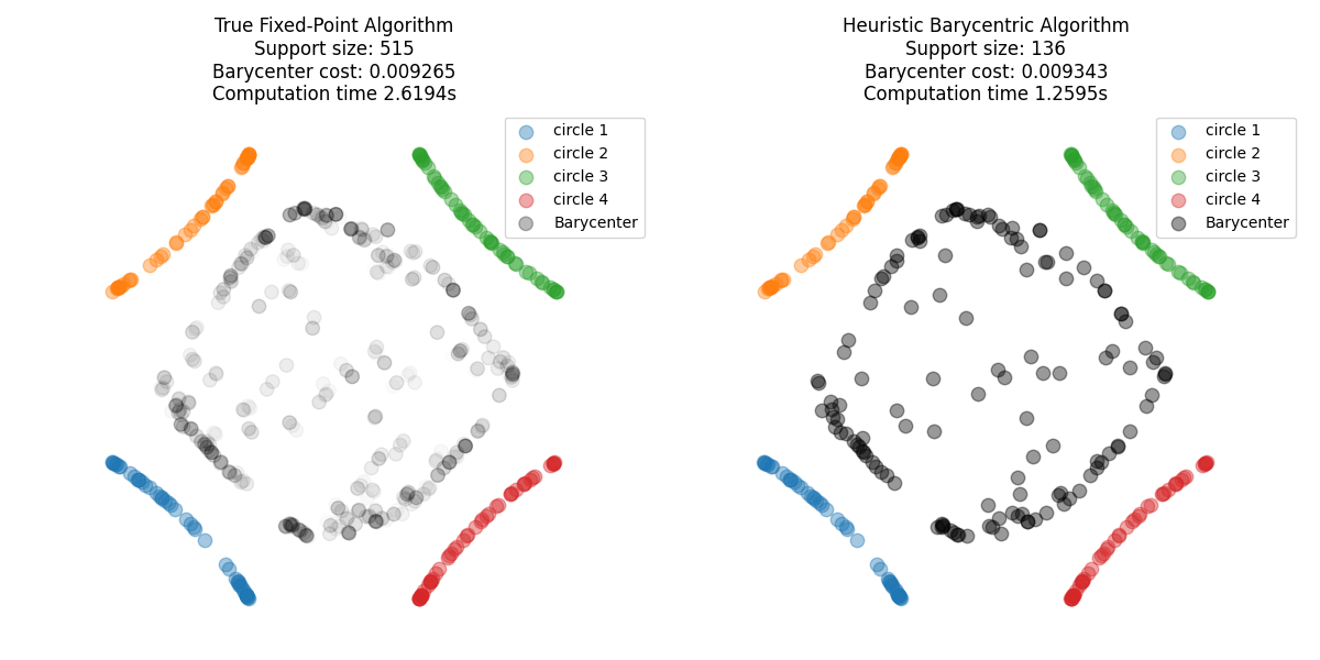
This example illustrates the computation of an Optimal Transport Barycenter for a ground cost that is not a power of a norm. We take the example of ground costs \(c_k(x, y) = \lambda_k\|P_k(x)-y\|_2^2\), where \(P_k\) is the (non-linear) projection onto a circle k, and \((\lambda_k)\) are weights. A barycenter is defined ([77]) as a minimiser of the energy \(V(\mu) = \sum_k \mathcal{T}_{c_k}(\mu, \nu_k)\) where \(\mu\) is a candidate barycenter measure, the measures \(\nu_k\) are the target measures and \(\mathcal{T}_{c_k}\) is the OT cost for ground cost \(c_k\). This is an example of the fixed-point barycenter solver introduced in [77] which generalises [20] and [43].

The ground barycenter function \(B(y_1, ..., y_K) = \mathrm{argmin}_{x \in \mathbb{R}^2} \sum_k \lambda_k c_k(x, y_k)\) is computed by gradient descent over \(x\) with Pytorch.

We compare two algorithms from [77]: the first ([77], Algorithm 2, ‘true_fixed_point’ in POT) has convergence guarantees but the iterations may increase in support size and thus require more computational resources. The second ([77], Algorithm 3, ‘L2_barycentric_proj’ in POT) is a simplified heuristic that imposes a fixed support size for the barycenter and fixed weights.

We initialise both algorithms with a support size of 136, computing a barycenter between measures with uniform weights and 50 points.

[77] Tanguy, Eloi and Delon, Julie and Gozlan, Nathaël (2024). Computing Barycentres of Measures for Generic Transport Costs. arXiv preprint 2501.04016 (2024)

[20] Cuturi, M. and Doucet, A. (2014) Fast Computation of Wasserstein Barycenters. InternationalConference in Machine Learning

[43] Álvarez-Esteban, Pedro C., et al. A fixed-point approach to barycenters in Wasserstein space. Journal of Mathematical Analysis and Applications 441.2 (2016): 744-762.

# Author: Eloi Tanguy <eloi.tanguy@math.cnrs.fr>
#
# License: MIT License

# sphinx_gallery_thumbnail_number = 1

Generate data

import torch
from torch.optim import Adam
from ot.utils import dist
import numpy as np
from ot.lp import free_support_barycenter_generic_costs
import matplotlib.pyplot as plt
from time import time


torch.manual_seed(42)

n = 136  # number of points of the barycentre
d = 2  # dimensions of the original measure
K = 4  # number of measures to barycentre
m_list = [49, 50, 51, 51]  # number of points of the measures
b_list = [torch.ones(m) / m for m in m_list]  # weights of the 4 measures
weights = torch.ones(K) / K  # weights for the barycentre
stop_threshold = 1e-20  # stop threshold for B and for fixed-point algo


# map R^2 -> R^2 projection onto circle
def proj_circle(X, origin, radius):
    diffs = X - origin[None, :]
    norms = torch.norm(diffs, dim=1)
    return origin[None, :] + radius * diffs / norms[:, None]


# circles on which to project
origin1 = torch.tensor([-1.0, -1.0])
origin2 = torch.tensor([-1.0, 2.0])
origin3 = torch.tensor([2.0, 2.0])
origin4 = torch.tensor([2.0, -1.0])
r = np.sqrt(2)
P_list = [
    lambda X: proj_circle(X, origin1, r),
    lambda X: proj_circle(X, origin2, r),
    lambda X: proj_circle(X, origin3, r),
    lambda X: proj_circle(X, origin4, r),
]

# measures to barycentre are projections of different random circles
# onto the K circles
Y_list = []
for k in range(K):
    t = torch.rand(m_list[k]) * 2 * np.pi
    X_temp = 0.5 * torch.stack([torch.cos(t), torch.sin(t)], axis=1)
    X_temp = X_temp + torch.tensor([0.5, 0.5])[None, :]
    Y_list.append(P_list[k](X_temp))

Define costs and ground barycenter function cost_list[k] is a function taking x (n, d) and y (n_k, d_k) and returning a (n, n_k) matrix of costs

def c1(x, y):
    return dist(P_list[0](x), y)


def c2(x, y):
    return dist(P_list[1](x), y)


def c3(x, y):
    return dist(P_list[2](x), y)


def c4(x, y):
    return dist(P_list[3](x), y)


cost_list = [c1, c2, c3, c4]


# batched total ground cost function for candidate points x (n, d)
# for computation of the ground barycenter B with gradient descent
def C(x, y):
    """
    Computes the barycenter cost for candidate points x (n, d) and
    measure supports y: List(n, d_k).
    """
    n = x.shape[0]
    K = len(y)
    out = torch.zeros(n)
    for k in range(K):
        out += (1 / K) * torch.sum((P_list[k](x) - y[k]) ** 2, axis=1)
    return out


# ground barycenter function
def B(y, its=150, lr=1, stop_threshold=stop_threshold):
    """
    Computes the ground barycenter for measure supports y: List(n, d_k).
    Output: (n, d) array
    """
    x = torch.randn(y[0].shape[0], d)
    x.requires_grad_(True)
    opt = Adam([x], lr=lr)
    for _ in range(its):
        x_prev = x.data.clone()
        opt.zero_grad()
        loss = torch.sum(C(x, y))
        loss.backward()
        opt.step()
        diff = torch.sum((x.data - x_prev) ** 2)
        if diff < stop_threshold:
            break
    return x

Compute the barycenter measure with the true fixed-point algorithm

fixed_point_its = 5
torch.manual_seed(42)
X_init = torch.rand(n, d)
t0 = time()
X_bar, a_bar, log_dict = free_support_barycenter_generic_costs(
    Y_list,
    b_list,
    X_init,
    cost_list,
    B,
    numItermax=fixed_point_its,
    stopThr=stop_threshold,
    method="true_fixed_point",
    log=True,
    clean_measure=True,
)
dt_true_fixed_point = time() - t0

Compute the barycenter measure with the barycentric (default) algorithm

fixed_point_its = 5
torch.manual_seed(42)
X_init = torch.rand(n, d)
t0 = time()
X_bar2, log_dict2 = free_support_barycenter_generic_costs(
    Y_list,
    b_list,
    X_init,
    cost_list,
    B,
    numItermax=fixed_point_its,
    stopThr=stop_threshold,
    log=True,
)
dt_barycentric = time() - t0

Plot Barycenters (Iteration 3)

alpha = 0.4
s = 80
labels = ["circle 1", "circle 2", "circle 3", "circle 4"]

fig, axes = plt.subplots(1, 2, figsize=(12, 6))

# Plot for the true fixed-point algorithm
for Y, label in zip(Y_list, labels):
    axes[0].scatter(*(Y.numpy()).T, alpha=alpha, label=label, s=s)
axes[0].scatter(
    *(X_bar.detach().numpy()).T,
    label="Barycenter",
    c="black",
    alpha=alpha * a_bar.numpy() / np.max(a_bar.numpy()),
    s=s,
)
axes[0].set_title(
    "True Fixed-Point Algorithm\n"
    f"Support size: {a_bar.shape[0]}\n"
    f"Barycenter cost: {log_dict['V_list'][-1].item():.6f}\n"
    f"Computation time {dt_true_fixed_point:.4f}s"
)
axes[0].axis("equal")
axes[0].axis("off")
axes[0].legend()

# Plot for the heuristic algorithm
for Y, label in zip(Y_list, labels):
    axes[1].scatter(*(Y.numpy()).T, alpha=alpha, label=label, s=s)
axes[1].scatter(
    *(X_bar2.detach().numpy()).T, label="Barycenter", c="black", alpha=alpha, s=s
)
axes[1].set_title(
    "Heuristic Barycentric Algorithm\n"
    f"Support size: {X_bar2.shape[0]}\n"
    f"Barycenter cost: {log_dict2['V_list'][-1].item():.6f}\n"
    f"Computation time {dt_barycentric:.4f}s"
)
axes[1].axis("equal")
axes[1].axis("off")
axes[1].legend()

plt.tight_layout()

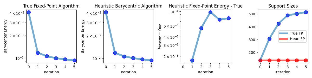
Plot energy convergence and support sizes

size = 3
n_plots = 4
fig, axes = plt.subplots(1, n_plots, figsize=(size * n_plots, size))
V_list = [V.item() for V in log_dict["V_list"]]
V_list2 = [V.item() for V in log_dict2["V_list"]]
diff = np.array(V_list2) - np.array(V_list)

# Plot for True Fixed-Point Algorithm
axes[0].plot(V_list, lw=5, alpha=0.6)
axes[0].scatter(range(len(V_list)), V_list, color="blue", alpha=0.8, s=100)
axes[0].set_title("True Fixed-Point Algorithm")
axes[0].set_xlabel("Iteration")
axes[0].set_ylabel("Barycenter Energy")
axes[0].set_yscale("log")
axes[0].xaxis.set_major_locator(plt.MaxNLocator(integer=True))

# Plot for Heuristic Barycentric Algorithm
axes[1].plot(V_list2, lw=5, alpha=0.6)
axes[1].scatter(range(len(V_list2)), V_list2, color="blue", alpha=0.8, s=100)
axes[1].set_title("Heuristic Barycentric Algorithm")
axes[1].set_xlabel("Iteration")
axes[1].set_ylabel("Barycenter Energy")
axes[1].set_yscale("log")
axes[1].xaxis.set_major_locator(plt.MaxNLocator(integer=True))

# Plot difference between the two
axes[2].plot(diff, lw=5, alpha=0.6)
axes[2].scatter(range(len(diff)), diff, color="blue", alpha=0.8, s=100)
axes[2].set_title("Heuristic Fixed-Point Energy - True")
axes[2].set_xlabel("Iteration")
axes[2].set_ylabel("$V_{\\mathrm{heuristic}} - V_{\\mathrm{true}}$")
axes[2].set_yscale("log")
axes[2].xaxis.set_major_locator(plt.MaxNLocator(integer=True))

# plot support sizes
support_sizes = [Xi.shape[0] for Xi in log_dict["X_list"]]
support_sizes2 = [Xi.shape[0] for Xi in log_dict2["X_list"]]

axes[3].plot(support_sizes, color="C0", lw=5, alpha=0.6, label="True FP")
axes[3].scatter(
    range(len(support_sizes)), support_sizes, color="blue", alpha=0.8, s=100
)
axes[3].plot(support_sizes2, color="red", lw=5, alpha=0.6, label="Heur. FP")
axes[3].scatter(
    range(len(support_sizes2)), support_sizes2, color="red", alpha=0.8, s=100
)
axes[3].legend(loc="best")
axes[3].set_xlabel("Iteration")
axes[3].xaxis.set_major_locator(plt.MaxNLocator(integer=True))
axes[3].set_title("Support Sizes")

plt.tight_layout()
plt.show()