Convolutional Wasserstein Barycenter example

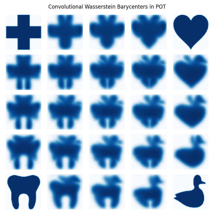
This example is designed to illustrate how the Convolutional Wasserstein Barycenter function of POT works.

# Author: Nicolas Courty <ncourty@irisa.fr>
#
# License: MIT License
import os
from pathlib import Path

import numpy as np
import matplotlib.pyplot as plt
import ot

Data preparation

The four distributions are constructed from 4 simple images

this_file = os.path.realpath("__file__")
data_path = os.path.join(Path(this_file).parent.parent.parent, "data")

f1 = 1 - plt.imread(os.path.join(data_path, "redcross.png"))[::2, ::2, 2]
f2 = 1 - plt.imread(os.path.join(data_path, "tooth.png"))[::2, ::2, 2]
f3 = 1 - plt.imread(os.path.join(data_path, "heart.png"))[::2, ::2, 2]
f4 = 1 - plt.imread(os.path.join(data_path, "duck.png"))[::2, ::2, 2]

f1 = f1 / np.sum(f1)
f2 = f2 / np.sum(f2)
f3 = f3 / np.sum(f3)
f4 = f4 / np.sum(f4)
A = np.array([f1, f2, f3, f4])

nb_images = 5

# those are the four corners coordinates that will be interpolated by bilinear
# interpolation
v1 = np.array((1, 0, 0, 0))
v2 = np.array((0, 1, 0, 0))
v3 = np.array((0, 0, 1, 0))
v4 = np.array((0, 0, 0, 1))

Barycenter computation and visualization

fig, axes = plt.subplots(nb_images, nb_images, figsize=(7, 7))
plt.suptitle("Convolutional Wasserstein Barycenters in POT")
cm = "Blues"
# regularization parameter
reg = 0.004
for i in range(nb_images):
    for j in range(nb_images):
        tx = float(i) / (nb_images - 1)
        ty = float(j) / (nb_images - 1)

        # weights are constructed by bilinear interpolation
        tmp1 = (1 - tx) * v1 + tx * v2
        tmp2 = (1 - tx) * v3 + tx * v4
        weights = (1 - ty) * tmp1 + ty * tmp2

        if i == 0 and j == 0:
            axes[i, j].imshow(f1, cmap=cm)
        elif i == 0 and j == (nb_images - 1):
            axes[i, j].imshow(f3, cmap=cm)
        elif i == (nb_images - 1) and j == 0:
            axes[i, j].imshow(f2, cmap=cm)
        elif i == (nb_images - 1) and j == (nb_images - 1):
            axes[i, j].imshow(f4, cmap=cm)
        else:
            # call to barycenter computation
            axes[i, j].imshow(
                ot.bregman.convolutional_barycenter2d(A, reg, weights), cmap=cm
            )
        axes[i, j].axis("off")
plt.tight_layout()
plt.show()