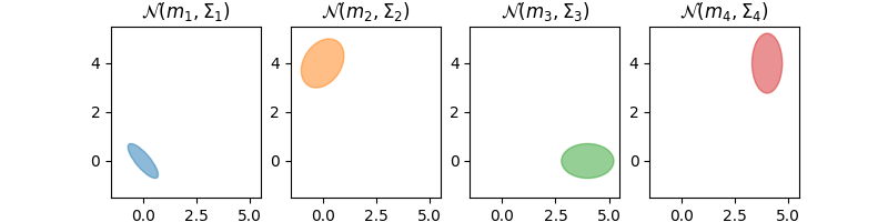
Gaussian Bures-Wasserstein barycenters

Illustration of Gaussian Bures-Wasserstein barycenters.

# Authors: Rémi Flamary <remi.flamary@polytechnique.edu>
#
# License: MIT License

# sphinx_gallery_thumbnail_number = 2

from matplotlib import colors
from matplotlib.patches import Ellipse
import numpy as np
import matplotlib.pylab as pl
import ot

Define Gaussian Covariances and distributions

C1 = np.array([[0.5, -0.4], [-0.4, 0.5]])
C2 = np.array([[1, 0.3], [0.3, 1]])
C3 = np.array([[1.5, 0], [0, 0.5]])
C4 = np.array([[0.5, 0], [0, 1.5]])

C = np.stack((C1, C2, C3, C4))

m1 = np.array([0, 0])
m2 = np.array([0, 4])
m3 = np.array([4, 0])
m4 = np.array([4, 4])

m = np.stack((m1, m2, m3, m4))

Plot the distributions

def draw_cov(mu, C, color=None, label=None, nstd=1):

    def eigsorted(cov):
        vals, vecs = np.linalg.eigh(cov)
        order = vals.argsort()[::-1]
        return vals[order], vecs[:, order]

    vals, vecs = eigsorted(C)
    theta = np.degrees(np.arctan2(*vecs[:, 0][::-1]))
    w, h = 2 * nstd * np.sqrt(vals)
    ell = Ellipse(xy=(mu[0], mu[1]),
                  width=w, height=h, alpha=0.5,
                  angle=theta, facecolor=color, edgecolor=color, label=label, fill=True)
    pl.gca().add_artist(ell)
    #pl.scatter(mu[0],mu[1],color=color, marker='x')


axis = [-1.5, 5.5, -1.5, 5.5]

pl.figure(1, (8, 2))
pl.clf()

pl.subplot(1, 4, 1)
draw_cov(m1, C1, color='C0')
pl.axis(axis)
pl.title('$\mathcal{N}(m_1,\Sigma_1)$')

pl.subplot(1, 4, 2)
draw_cov(m2, C2, color='C1')
pl.axis(axis)
pl.title('$\mathcal{N}(m_2,\Sigma_2)$')

pl.subplot(1, 4, 3)
draw_cov(m3, C3, color='C2')
pl.axis(axis)
pl.title('$\mathcal{N}(m_3,\Sigma_3)$')

pl.subplot(1, 4, 4)
draw_cov(m4, C4, color='C3')
pl.axis(axis)
pl.title('$\mathcal{N}(m_4,\Sigma_4)$')

Text(0.5, 1.0, '$\\mathcal{N}(m_4,\\Sigma_4)$')

Compute Bures-Wasserstein barycenters and plot them

# basis for bilinear interpolation
v1 = np.array((1, 0, 0, 0))
v2 = np.array((0, 1, 0, 0))
v3 = np.array((0, 0, 1, 0))
v4 = np.array((0, 0, 0, 1))


colors = np.stack((colors.to_rgb('C0'),
                   colors.to_rgb('C1'),
                   colors.to_rgb('C2'),
                   colors.to_rgb('C3')))

pl.figure(2, (8, 8))

nb_interp = 6

for i in range(nb_interp):
    for j in range(nb_interp):
        tx = float(i) / (nb_interp - 1)
        ty = float(j) / (nb_interp - 1)

        # weights are constructed by bilinear interpolation
        tmp1 = (1 - tx) * v1 + tx * v2
        tmp2 = (1 - tx) * v3 + tx * v4
        weights = (1 - ty) * tmp1 + ty * tmp2

        color = np.dot(colors.T, weights)

        mb, Cb = ot.gaussian.bures_wasserstein_barycenter(m, C, weights)

        draw_cov(mb, Cb, color=color, label=None, nstd=0.3)

pl.axis(axis)
pl.axis('off')
pl.tight_layout()