OT for image color adaptation with mapping estimation

Note

Example added in release: 0.1.9.

OT for domain adaptation with image color adaptation [6] with mapping estimation [8].

[6] Ferradans, S., Papadakis, N., Peyre, G., & Aujol, J. F. (2014). Regularized discrete optimal transport. SIAM Journal on Imaging Sciences, 7(3), 1853-1882.

[8] M. Perrot, N. Courty, R. Flamary, A. Habrard, “Mapping estimation for discrete optimal transport”, Neural Information Processing Systems (NIPS), 2016.

# Authors: Remi Flamary <remi.flamary@unice.fr>
#          Stanislas Chambon <stan.chambon@gmail.com>
#
# License: MIT License

# sphinx_gallery_thumbnail_number = 3
import os
from pathlib import Path

import numpy as np
from matplotlib import pyplot as plt
import ot

rng = np.random.RandomState(42)


def im2mat(img):
    """Converts and image to matrix (one pixel per line)"""
    return img.reshape((img.shape[0] * img.shape[1], img.shape[2]))


def mat2im(X, shape):
    """Converts back a matrix to an image"""
    return X.reshape(shape)


def minmax(img):
    return np.clip(img, 0, 1)

Generate data

# Loading images
this_file = os.path.realpath("__file__")
data_path = os.path.join(Path(this_file).parent.parent.parent, "data")

I1 = plt.imread(os.path.join(data_path, "ocean_day.jpg")).astype(np.float64) / 256
I2 = plt.imread(os.path.join(data_path, "ocean_sunset.jpg")).astype(np.float64) / 256

X1 = im2mat(I1)
X2 = im2mat(I2)

# training samples
nb = 500
idx1 = rng.randint(X1.shape[0], size=(nb,))
idx2 = rng.randint(X2.shape[0], size=(nb,))

Xs = X1[idx1, :]
Xt = X2[idx2, :]

Domain adaptation for pixel distribution transfer

# EMDTransport
ot_emd = ot.da.EMDTransport()
ot_emd.fit(Xs=Xs, Xt=Xt)
transp_Xs_emd = ot_emd.transform(Xs=X1)
Image_emd = minmax(mat2im(transp_Xs_emd, I1.shape))

# SinkhornTransport
ot_sinkhorn = ot.da.SinkhornTransport(reg_e=1e-1)
ot_sinkhorn.fit(Xs=Xs, Xt=Xt)
transp_Xs_sinkhorn = ot_sinkhorn.transform(Xs=X1)
Image_sinkhorn = minmax(mat2im(transp_Xs_sinkhorn, I1.shape))

ot_mapping_linear = ot.da.MappingTransport(
    mu=1e0, eta=1e-8, bias=True, max_iter=20, verbose=True
)
ot_mapping_linear.fit(Xs=Xs, Xt=Xt)

X1tl = ot_mapping_linear.transform(Xs=X1)
Image_mapping_linear = minmax(mat2im(X1tl, I1.shape))

ot_mapping_gaussian = ot.da.MappingTransport(
    mu=1e0, eta=1e-2, sigma=1, bias=False, max_iter=10, verbose=True
)
ot_mapping_gaussian.fit(Xs=Xs, Xt=Xt)

X1tn = ot_mapping_gaussian.transform(Xs=X1)  # use the estimated mapping
Image_mapping_gaussian = minmax(mat2im(X1tn, I1.shape))

It.  |Loss        |Delta loss
--------------------------------
    0|1.797241e+02|0.000000e+00
    1|1.758006e+02|-2.183097e-02
    2|1.757017e+02|-5.624432e-04
    3|1.756517e+02|-2.849028e-04
    4|1.756213e+02|-1.730169e-04
    5|1.756010e+02|-1.153554e-04
    6|1.755867e+02|-8.145467e-05
    7|1.755758e+02|-6.191708e-05
    8|1.755672e+02|-4.887528e-05
    9|1.755603e+02|-3.940598e-05
   10|1.755547e+02|-3.221693e-05
   11|1.755499e+02|-2.695124e-05
   12|1.755460e+02|-2.267882e-05
   13|1.755425e+02|-1.978388e-05
   14|1.755395e+02|-1.727352e-05
   15|1.755368e+02|-1.507117e-05
   16|1.755345e+02|-1.332464e-05
   17|1.755324e+02|-1.192166e-05
   18|1.755310e+02|-7.621166e-06
It.  |Loss        |Delta loss
--------------------------------
    0|1.841990e+02|0.000000e+00
    1|1.780133e+02|-3.358178e-02
    2|1.778463e+02|-9.378722e-04
    3|1.777836e+02|-3.528609e-04
    4|1.777494e+02|-1.920544e-04
    5|1.777281e+02|-1.203681e-04
    6|1.777133e+02|-8.319697e-05
    7|1.777027e+02|-5.969768e-05
    8|1.776945e+02|-4.608957e-05
    9|1.776880e+02|-3.652085e-05
   10|1.776828e+02|-2.929145e-05

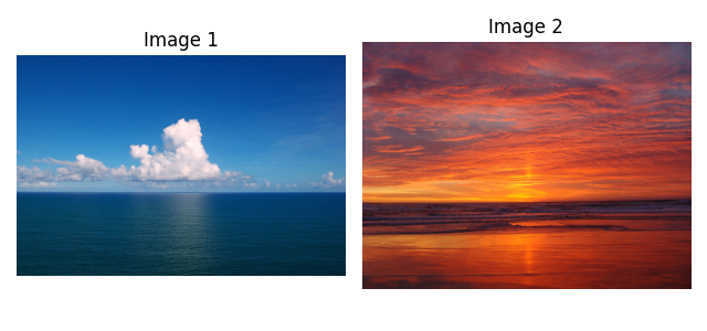
Plot original images

plt.figure(1, figsize=(6.4, 3))
plt.subplot(1, 2, 1)
plt.imshow(I1)
plt.axis("off")
plt.title("Image 1")

plt.subplot(1, 2, 2)
plt.imshow(I2)
plt.axis("off")
plt.title("Image 2")
plt.tight_layout()

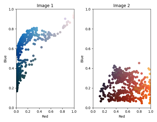
Plot pixel values distribution

plt.figure(2, figsize=(6.4, 5))

plt.subplot(1, 2, 1)
plt.scatter(Xs[:, 0], Xs[:, 2], c=Xs)
plt.axis([0, 1, 0, 1])
plt.xlabel("Red")
plt.ylabel("Blue")
plt.title("Image 1")

plt.subplot(1, 2, 2)
plt.scatter(Xt[:, 0], Xt[:, 2], c=Xt)
plt.axis([0, 1, 0, 1])
plt.xlabel("Red")
plt.ylabel("Blue")
plt.title("Image 2")
plt.tight_layout()

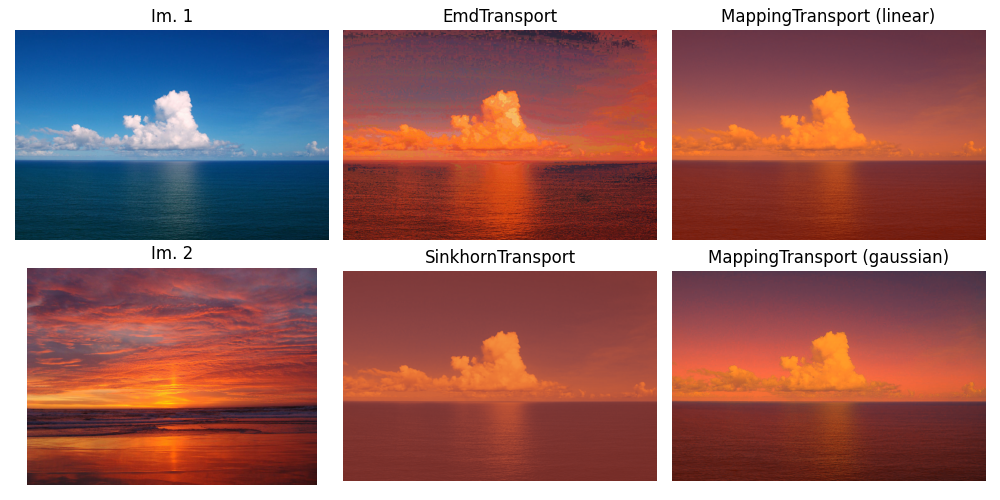
Plot transformed images

plt.figure(2, figsize=(10, 5))

plt.subplot(2, 3, 1)
plt.imshow(I1)
plt.axis("off")
plt.title("Im. 1")

plt.subplot(2, 3, 4)
plt.imshow(I2)
plt.axis("off")
plt.title("Im. 2")

plt.subplot(2, 3, 2)
plt.imshow(Image_emd)
plt.axis("off")
plt.title("EmdTransport")

plt.subplot(2, 3, 5)
plt.imshow(Image_sinkhorn)
plt.axis("off")
plt.title("SinkhornTransport")

plt.subplot(2, 3, 3)
plt.imshow(Image_mapping_linear)
plt.axis("off")
plt.title("MappingTransport (linear)")

plt.subplot(2, 3, 6)
plt.imshow(Image_mapping_gaussian)
plt.axis("off")
plt.title("MappingTransport (gaussian)")
plt.tight_layout()

plt.show()