Solve Fused Unbalanced Gromov Wasserstein with Adam

Since the FUGW loss is differentiable, it can be minimized with first-order optimization. We show how to do this with the loss_fugw_batch function and compare the results with the dedicated FUGW solver fused_unbalanced_gromov_wasserstein.

# Author: Rémi Flamary <remi.flamary@polytechnique.edu>
#         Sonia Mazelet <sonia.mazelet@polytechnique.edu>
#
# License: MIT License

# sphinx_gallery_thumbnail_number = 3

import numpy as np
import matplotlib.pylab as pl
import torch
from time import perf_counter
import ot
from ot.batch._quadratic import loss_quadratic_batch, tensor_batch
from ot.gromov import fused_unbalanced_gromov_wasserstein
from sklearn.manifold import MDS

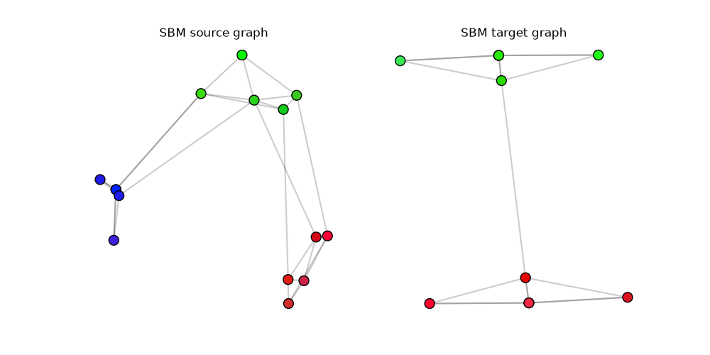
Generation of source and target graphs

rng = np.random.RandomState(42)


def get_sbm(n, nc, ratio, P):
    nbpc = np.round(n * ratio).astype(int)
    n = np.sum(nbpc)
    C = np.zeros((n, n))
    for c1 in range(nc):
        for c2 in range(c1 + 1):
            if c1 == c2:
                for i in range(np.sum(nbpc[:c1]), np.sum(nbpc[: c1 + 1])):
                    for j in range(np.sum(nbpc[:c2]), i):
                        if rng.rand() <= P[c1, c2]:
                            C[i, j] = 1
            else:
                for i in range(np.sum(nbpc[:c1]), np.sum(nbpc[: c1 + 1])):
                    for j in range(np.sum(nbpc[:c2]), np.sum(nbpc[: c2 + 1])):
                        if rng.rand() <= P[c1, c2]:
                            C[i, j] = 1

    return C + C.T


def plot_graph(x, C, color="C0", s=100):
    for j in range(C.shape[0]):
        for i in range(j):
            if C[i, j] > 0:
                pl.plot([x[i, 0], x[j, 0]], [x[i, 1], x[j, 1]], alpha=0.2, color="k")
    pl.scatter(x[:, 0], x[:, 1], c=color, s=s, zorder=10, edgecolors="k")


def get_sbm_labels(n, ratio):
    nbpc = np.round(n * ratio).astype(int)
    return np.concatenate(
        [np.full(count, label, dtype=int) for label, count in enumerate(nbpc)]
    )


def get_noisy_one_hot(labels, n_classes, noise_level=0.1):
    x = np.eye(n_classes)[labels]
    x += noise_level * rng.randn(*x.shape)
    return x


n1 = 15
n2 = 10
nc1 = 3
nc2 = 2
ratio1 = np.array([0.33, 0.33, 0.33])
ratio2 = np.array([0.5, 0.5])

P1 = np.array([[0.8, 0.03, 0.0], [0.08, 0.8, 0.03], [0.0, 0.08, 0.8]])
P2 = np.array(0.8 * np.eye(2) + 0.01 * np.ones((2, 2)))
C1 = get_sbm(n1, nc1, ratio1, P1)
C2 = get_sbm(n2, nc2, ratio2, P2)
labels1 = get_sbm_labels(n1, ratio1)
labels2 = get_sbm_labels(n2, ratio2)

# Use noisy one-hot encodings of the SBM classes as node features.
feature_dim = max(nc1, nc2)
x1 = get_noisy_one_hot(labels1, feature_dim)
x2 = get_noisy_one_hot(labels2, feature_dim)
all_features = np.vstack([x1, x2])
feature_min = all_features[:, :3].min(axis=0, keepdims=True)
feature_max = all_features[:, :3].max(axis=0, keepdims=True)

# get 2d positions for visualization
pos1 = MDS(dissimilarity="precomputed", random_state=0, n_init=1).fit_transform(1 - C1)
pos2 = MDS(dissimilarity="precomputed", random_state=0, n_init=1).fit_transform(1 - C2)

colors1 = np.clip(
    (x1 - feature_min) / np.maximum(feature_max - feature_min, 1e-15), 0.0, 1.0
)
colors2 = np.clip(
    (x2 - feature_min) / np.maximum(feature_max - feature_min, 1e-15), 0.0, 1.0
)


pl.figure(1, (10, 5))
pl.clf()
pl.subplot(1, 2, 1)
plot_graph(pos1, C1, color=colors1)
pl.title("SBM source graph")
pl.axis("off")
pl.subplot(1, 2, 2)
plot_graph(pos2, C2, color=colors2)
pl.title("SBM target graph")
_ = pl.axis("off")

/home/circleci/.local/lib/python3.12/site-packages/sklearn/manifold/_mds.py:735: FutureWarning: The default value of `init` will change from 'random' to 'classical_mds' in 1.10. To suppress this warning, provide some value of `init`.
  warnings.warn(
/home/circleci/.local/lib/python3.12/site-packages/sklearn/manifold/_mds.py:752: FutureWarning: The `dissimilarity` parameter is deprecated and will be removed in 1.10. Use `metric` instead.
  warnings.warn(
/home/circleci/.local/lib/python3.12/site-packages/sklearn/manifold/_mds.py:735: FutureWarning: The default value of `init` will change from 'random' to 'classical_mds' in 1.10. To suppress this warning, provide some value of `init`.
  warnings.warn(
/home/circleci/.local/lib/python3.12/site-packages/sklearn/manifold/_mds.py:752: FutureWarning: The `dissimilarity` parameter is deprecated and will be removed in 1.10. Use `metric` instead.
  warnings.warn(

Solve FUGW with Adam

# Even though `loss_fugw_batch` supports batches of problems, we use a
# batch of size 1 here for clarity.

a = ot.unif(C1.shape[0])
b = ot.unif(C2.shape[0])
M = ot.dist(x1, x2)
M /= M.max()

a_torch = torch.tensor(a[None, :])
b_torch = torch.tensor(b[None, :])
C1_torch = torch.tensor(C1[None, :, :])
C2_torch = torch.tensor(C2[None, :, :])
M_torch = torch.tensor(M[None, :, :])
L = tensor_batch(a_torch, b_torch, C1_torch, C2_torch, loss="sqeuclidean")

alpha = 0.5
reg_marginals = 0.5
lr = 5e-2
nb_iter_max = 1500
tol = 1e-7

T0_torch = a_torch[:, :, None] * b_torch[:, None, :]
T_torch = torch.log(torch.expm1(T0_torch)).clone().requires_grad_(True)
optimizer = torch.optim.Adam([T_torch], lr=lr)
loss_iter = []
mass_iter = []
previous_plan_torch = None

tic = perf_counter()
for i in range(nb_iter_max):
    optimizer.zero_grad()
    # Positive transport plan parameterized as log(1 + exp(T)).
    plan_torch = torch.nn.functional.softplus(T_torch)
    loss = loss_quadratic_batch(
        a_torch,
        b_torch,
        C1_torch,
        C2_torch,
        plan_torch,
        M_torch,
        alpha=alpha,
        unbalanced=reg_marginals,
        unbalanced_type="kl",
        recompute_const=True,
    )[0]

    loss_iter.append(float(loss.detach()))
    mass_iter.append(float(plan_torch.detach().sum()))
    if previous_plan_torch is not None:
        err = float(torch.sum(torch.abs(plan_torch.detach() - previous_plan_torch)))
        if err < tol:
            break
    previous_plan_torch = plan_torch.detach().clone()
    loss.backward()
    optimizer.step()
time_adam = perf_counter() - tic

T_adam = torch.nn.functional.softplus(T_torch).detach().cpu().numpy()[0]

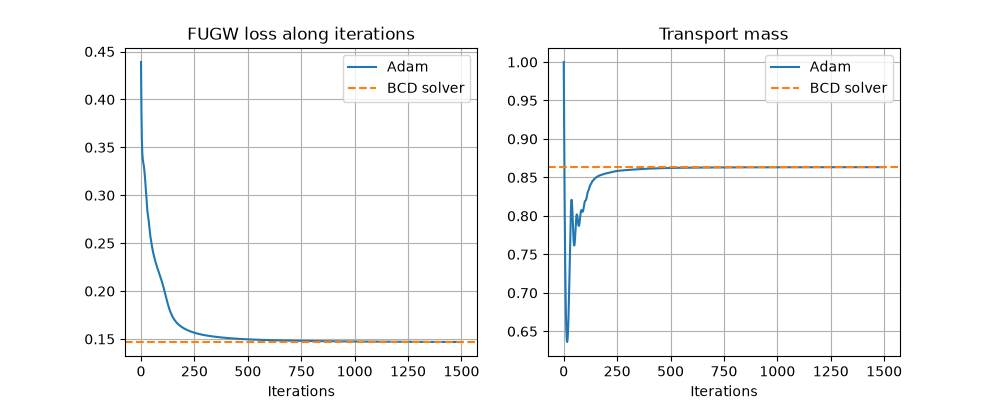
Compare with the dedicated FUGW solver

The dedicated solver uses a block coordinate descent (BCD) scheme. We compare the coupling it returns with the one obtained by direct Adam minimization of loss_fugw_batch.

def evaluate_batch_fugw_loss(plan):
    plan_torch = torch.tensor(plan[None, :, :], dtype=M_torch.dtype)
    loss = loss_quadratic_batch(
        a_torch,
        b_torch,
        C1_torch,
        C2_torch,
        plan_torch,
        M_torch,
        alpha=alpha,
        unbalanced=reg_marginals,
        unbalanced_type="kl",
        recompute_const=True,
    )[0]
    return float(loss.detach())


tic = perf_counter()
result = ot.solve_gromov(
    C1, C2, M, a, b, alpha=alpha, reg=0, unbalanced_type="kl", unbalanced=reg_marginals
)
time_bcd = perf_counter() - tic

loss_adam_final = evaluate_batch_fugw_loss(T_adam)
T_bcd = result.plan
loss_bcd_final = evaluate_batch_fugw_loss(T_bcd)
mass_bcd = T_bcd.sum()

pl.figure(2, (10, 4))
pl.clf()
pl.subplot(1, 2, 1)
pl.plot(loss_iter, label="Adam")
pl.axhline(loss_bcd_final, color="C1", linestyle="--", label="BCD solver")
pl.grid()
pl.title("FUGW loss along iterations")
pl.xlabel("Iterations")
pl.legend()
pl.subplot(1, 2, 2)
pl.plot(mass_iter, label="Adam")
pl.axhline(mass_bcd, color="C1", linestyle="--", label="BCD solver")
pl.grid()
pl.title("Transport mass")
pl.xlabel("Iterations")
_ = pl.legend()

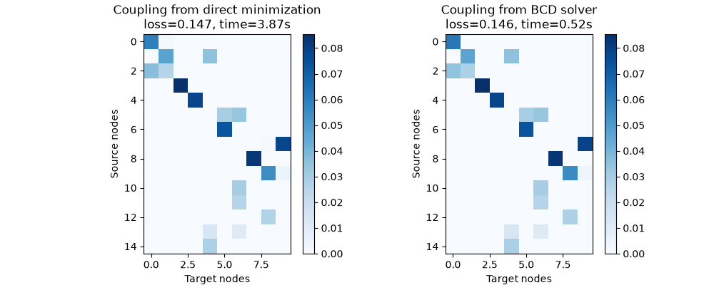
Visualize the learned couplings

We visualize the couplings obtained by both methods to compare them. On this example, both methods recover similar couplings, but direct minimization reaches a lower loss_fugw_batch value at the cost of a longer runtime.

vmin = min(T_adam.min(), T_bcd.min())
vmax = max(T_adam.max(), T_bcd.max())
pl.figure(3, (10, 4))
pl.clf()
pl.subplot(1, 2, 1)
pl.imshow(T_adam, interpolation="nearest", cmap="Blues", vmin=vmin, vmax=vmax)
pl.title(
    f"Coupling from direct minimization\nloss={loss_adam_final:.3f}, time={time_adam:.2f}s"
)
pl.xlabel("Target nodes")
pl.ylabel("Source nodes")
pl.colorbar()
pl.subplot(1, 2, 2)
pl.imshow(T_bcd, interpolation="nearest", cmap="Blues", vmin=vmin, vmax=vmax)
pl.title(f"Coupling from BCD solver\nloss={loss_bcd_final:.3f}, time={time_bcd:.2f}s")
pl.xlabel("Target nodes")
pl.ylabel("Source nodes")
_ = pl.colorbar()