Sliced Wasserstein barycenter and gradient flow with PyTorch

Note

Example added in release: 0.8.0.

In this example we use the pytorch backend to optimize the sliced Wasserstein loss between two empirical distributions [31].

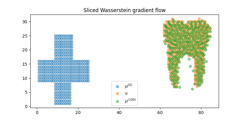
In the first example one we perform a gradient flow on the support of a distribution that minimize the sliced Wasserstein distance as proposed in [36].

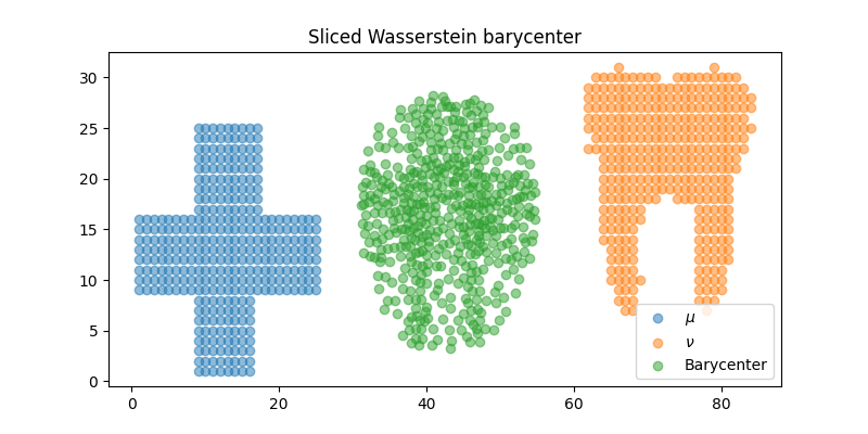
In the second example we optimize with a gradient descent the sliced Wasserstein barycenter between two distributions as in [31].

[31] Bonneel, Nicolas, et al. “Sliced and radon wasserstein barycenters of measures.” Journal of Mathematical Imaging and Vision 51.1 (2015): 22-45

[36] Liutkus, A., Simsekli, U., Majewski, S., Durmus, A., & Stöter, F. R. (2019, May). Sliced-Wasserstein flows: Nonparametric generative modeling via optimal transport and diffusions. In International Conference on Machine Learning (pp. 4104-4113). PMLR.

# Author: Rémi Flamary <remi.flamary@polytechnique.edu>
#
# License: MIT License

# sphinx_gallery_thumbnail_number = 4

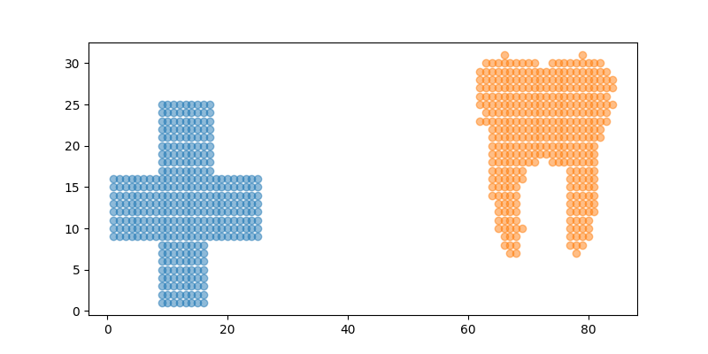
Loading the data

import numpy as np
import matplotlib.pylab as pl
import torch
import ot
import matplotlib.animation as animation

I1 = pl.imread("../../data/redcross.png").astype(np.float64)[::5, ::5, 2]
I2 = pl.imread("../../data/tooth.png").astype(np.float64)[::5, ::5, 2]

sz = I2.shape[0]
XX, YY = np.meshgrid(np.arange(sz), np.arange(sz))

x1 = np.stack((XX[I1 == 0], YY[I1 == 0]), 1) * 1.0
x2 = np.stack((XX[I2 == 0] + 60, -YY[I2 == 0] + 32), 1) * 1.0
x3 = np.stack((XX[I2 == 0], -YY[I2 == 0] + 32), 1) * 1.0

pl.figure(1, (8, 4))
pl.scatter(x1[:, 0], x1[:, 1], alpha=0.5)
pl.scatter(x2[:, 0], x2[:, 1], alpha=0.5)

<matplotlib.collections.PathCollection object at 0x7fcfec776530>

Sliced Wasserstein gradient flow with Pytorch

device = "cuda" if torch.cuda.is_available() else "cpu"

# use pyTorch for our data
x1_torch = torch.tensor(x1).to(device=device).requires_grad_(True)
x2_torch = torch.tensor(x2).to(device=device)


lr = 1e3
nb_iter_max = 50

x_all = np.zeros((nb_iter_max, x1.shape[0], 2))

loss_iter = []

# generator for random permutations
gen = torch.Generator(device=device)
gen.manual_seed(42)

for i in range(nb_iter_max):
    loss = ot.sliced_wasserstein_distance(
        x1_torch, x2_torch, n_projections=20, seed=gen
    )

    loss_iter.append(loss.clone().detach().cpu().numpy())
    loss.backward()

    # performs a step of projected gradient descent
    with torch.no_grad():
        grad = x1_torch.grad
        x1_torch -= grad * lr / (1 + i / 5e1)  # step
        x1_torch.grad.zero_()
        x_all[i, :, :] = x1_torch.clone().detach().cpu().numpy()

xb = x1_torch.clone().detach().cpu().numpy()

pl.figure(2, (8, 4))
pl.scatter(x1[:, 0], x1[:, 1], alpha=0.5, label="$\mu^{(0)}$")
pl.scatter(x2[:, 0], x2[:, 1], alpha=0.5, label=r"$\nu$")
pl.scatter(xb[:, 0], xb[:, 1], alpha=0.5, label="$\mu^{(100)}$")
pl.title("Sliced Wasserstein gradient flow")
pl.legend()
ax = pl.axis()

Animate trajectories of the gradient flow along iteration

pl.figure(3, (8, 4))


def _update_plot(i):
    pl.clf()
    pl.scatter(x1[:, 0], x1[:, 1], alpha=0.5, label="$\mu^{(0)}$")
    pl.scatter(x2[:, 0], x2[:, 1], alpha=0.5, label=r"$\nu$")
    pl.scatter(x_all[i, :, 0], x_all[i, :, 1], alpha=0.5, label="$\mu^{(100)}$")
    pl.title("Sliced Wasserstein gradient flow Iter. {}".format(i))
    pl.axis(ax)
    return 1


ani = animation.FuncAnimation(
    pl.gcf(), _update_plot, nb_iter_max, interval=100, repeat_delay=2000
)

Once Loop Reflect

Compute the Sliced Wasserstein Barycenter

x1_torch = torch.tensor(x1).to(device=device)
x3_torch = torch.tensor(x3).to(device=device)
xbinit = np.random.randn(500, 2) * 10 + 16
xbary_torch = torch.tensor(xbinit).to(device=device).requires_grad_(True)

lr = 1e3
nb_iter_max = 50

x_all = np.zeros((nb_iter_max, xbary_torch.shape[0], 2))

loss_iter = []

# generator for random permutations
gen = torch.Generator(device=device)
gen.manual_seed(42)

alpha = 0.5

for i in range(nb_iter_max):
    loss = alpha * ot.sliced_wasserstein_distance(
        xbary_torch, x3_torch, n_projections=50, seed=gen
    ) + (1 - alpha) * ot.sliced_wasserstein_distance(
        xbary_torch, x1_torch, n_projections=50, seed=gen
    )

    loss_iter.append(loss.clone().detach().cpu().numpy())
    loss.backward()

    # performs a step of projected gradient descent
    with torch.no_grad():
        grad = xbary_torch.grad
        xbary_torch -= grad * lr  # / (1 + i / 5e1)  # step
        xbary_torch.grad.zero_()
        x_all[i, :, :] = xbary_torch.clone().detach().cpu().numpy()

xb = xbary_torch.clone().detach().cpu().numpy()

pl.figure(4, (8, 4))
pl.scatter(x1[:, 0], x1[:, 1], alpha=0.5, label="$\mu$")
pl.scatter(x2[:, 0], x2[:, 1], alpha=0.5, label=r"$\nu$")
pl.scatter(xb[:, 0] + 30, xb[:, 1], alpha=0.5, label="Barycenter")
pl.title("Sliced Wasserstein barycenter")
pl.legend()
ax = pl.axis()

Animate trajectories of the barycenter along gradient descent

pl.figure(5, (8, 4))


def _update_plot(i):
    pl.clf()
    pl.scatter(x1[:, 0], x1[:, 1], alpha=0.5, label="$\mu^{(0)}$")
    pl.scatter(x2[:, 0], x2[:, 1], alpha=0.5, label=r"$\nu$")
    pl.scatter(x_all[i, :, 0] + 30, x_all[i, :, 1], alpha=0.5, label="$\mu^{(100)}$")
    pl.title("Sliced Wasserstein barycenter Iter. {}".format(i))
    pl.axis(ax)
    return 1


ani = animation.FuncAnimation(
    pl.gcf(), _update_plot, nb_iter_max, interval=100, repeat_delay=2000
)

Once Loop Reflect