Dual OT solvers for entropic and quadratic regularized OT with Pytorch

# Author: Remi Flamary <remi.flamary@polytechnique.edu>
#
# License: MIT License

# sphinx_gallery_thumbnail_number = 3

import numpy as np
import matplotlib.pyplot as pl
import torch
import ot
import ot.plot

Data generation

torch.manual_seed(1)

n_source_samples = 100
n_target_samples = 100
theta = 2 * np.pi / 20
noise_level = 0.1

Xs, ys = ot.datasets.make_data_classif("gaussrot", n_source_samples, nz=noise_level)
Xt, yt = ot.datasets.make_data_classif(
    "gaussrot", n_target_samples, theta=theta, nz=noise_level
)

# one of the target mode changes its variance (no linear mapping)
Xt[yt == 2] *= 3
Xt = Xt + 4

Plot data

pl.figure(1, (10, 5))
pl.clf()
pl.scatter(Xs[:, 0], Xs[:, 1], marker="+", label="Source samples")
pl.scatter(Xt[:, 0], Xt[:, 1], marker="o", label="Target samples")
pl.legend(loc=0)
pl.title("Source and target distributions")

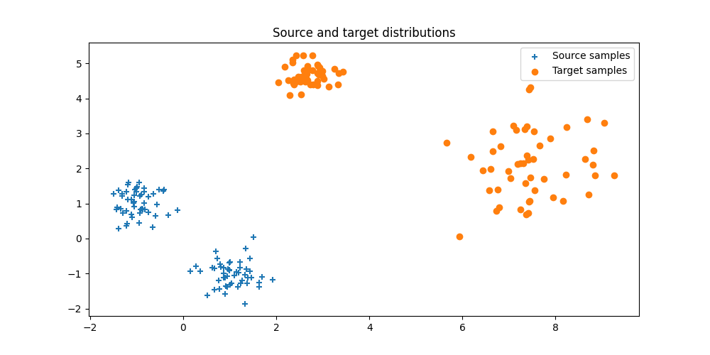
Text(0.5, 1.0, 'Source and target distributions')

Convert data to torch tensors

xs = torch.tensor(Xs)
xt = torch.tensor(Xt)

Estimating dual variables for entropic OT

u = torch.randn(n_source_samples, requires_grad=True)
v = torch.randn(n_source_samples, requires_grad=True)

reg = 0.5

optimizer = torch.optim.Adam([u, v], lr=1)

# number of iteration
n_iter = 200


losses = []

for i in range(n_iter):
    # generate noise samples

    # minus because we maximize the dual loss
    loss = -ot.stochastic.loss_dual_entropic(u, v, xs, xt, reg=reg)
    losses.append(float(loss.detach()))

    if i % 10 == 0:
        print("Iter: {:3d}, loss={}".format(i, losses[-1]))

    loss.backward()
    optimizer.step()
    optimizer.zero_grad()


pl.figure(2)
pl.plot(losses)
pl.grid()
pl.title("Dual objective (negative)")
pl.xlabel("Iterations")

Ge = ot.stochastic.plan_dual_entropic(u, v, xs, xt, reg=reg)

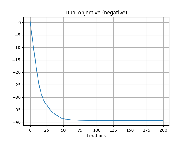
Iter:   0, loss=0.20204949002247385
Iter:  10, loss=-19.598840195117187
Iter:  20, loss=-31.45275877977004
Iter:  30, loss=-35.654959166703776
Iter:  40, loss=-38.55564856024449
Iter:  50, loss=-40.616177419309466
Iter:  60, loss=-41.31875285406105
Iter:  70, loss=-41.67965100682904
Iter:  80, loss=-41.869261766871475
Iter:  90, loss=-41.90013973873414
Iter: 100, loss=-41.932317369414754
Iter: 110, loss=-41.94220449340273
Iter: 120, loss=-41.950364300815394
Iter: 130, loss=-41.953795308746166
Iter: 140, loss=-41.95599677401932
Iter: 150, loss=-41.957543840951914
Iter: 160, loss=-41.95855874663437
Iter: 170, loss=-41.959284820103846
Iter: 180, loss=-41.959815373763206
Iter: 190, loss=-41.960213442186

Plot the estimated entropic OT plan

pl.figure(3, (10, 5))
pl.clf()
ot.plot.plot2D_samples_mat(Xs, Xt, Ge.detach().numpy(), alpha=0.1)
pl.scatter(Xs[:, 0], Xs[:, 1], marker="+", label="Source samples", zorder=2)
pl.scatter(Xt[:, 0], Xt[:, 1], marker="o", label="Target samples", zorder=2)
pl.legend(loc=0)
pl.title("Source and target distributions")

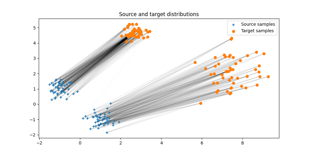
Text(0.5, 1.0, 'Source and target distributions')

Estimating dual variables for quadratic OT

u = torch.randn(n_source_samples, requires_grad=True)
v = torch.randn(n_source_samples, requires_grad=True)

reg = 0.01

optimizer = torch.optim.Adam([u, v], lr=1)

# number of iteration
n_iter = 200


losses = []


for i in range(n_iter):
    # generate noise samples

    # minus because we maximize the dual loss
    loss = -ot.stochastic.loss_dual_quadratic(u, v, xs, xt, reg=reg)
    losses.append(float(loss.detach()))

    if i % 10 == 0:
        print("Iter: {:3d}, loss={}".format(i, losses[-1]))

    loss.backward()
    optimizer.step()
    optimizer.zero_grad()


pl.figure(4)
pl.plot(losses)
pl.grid()
pl.title("Dual objective (negative)")
pl.xlabel("Iterations")

Gq = ot.stochastic.plan_dual_quadratic(u, v, xs, xt, reg=reg)

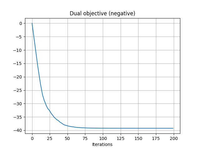
Iter:   0, loss=-0.0018442196020623663
Iter:  10, loss=-19.482693753355026
Iter:  20, loss=-31.031587667901338
Iter:  30, loss=-35.24412455339648
Iter:  40, loss=-38.34167509988665
Iter:  50, loss=-40.33264368175991
Iter:  60, loss=-41.05848772529333
Iter:  70, loss=-41.498203806732256
Iter:  80, loss=-41.701770668580316
Iter:  90, loss=-41.75788169087051
Iter: 100, loss=-41.78912743553177
Iter: 110, loss=-41.80275113616942
Iter: 120, loss=-41.81127971513494
Iter: 130, loss=-41.81620688759422
Iter: 140, loss=-41.81919900711129
Iter: 150, loss=-41.82131280293244
Iter: 160, loss=-41.82282129129657
Iter: 170, loss=-41.823959203849064
Iter: 180, loss=-41.82483864631298
Iter: 190, loss=-41.825524003745045

Plot the estimated quadratic OT plan

pl.figure(5, (10, 5))
pl.clf()
ot.plot.plot2D_samples_mat(Xs, Xt, Gq.detach().numpy(), alpha=0.1)
pl.scatter(Xs[:, 0], Xs[:, 1], marker="+", label="Source samples", zorder=2)
pl.scatter(Xt[:, 0], Xt[:, 1], marker="o", label="Target samples", zorder=2)
pl.legend(loc=0)
pl.title("OT plan with quadratic regularization")

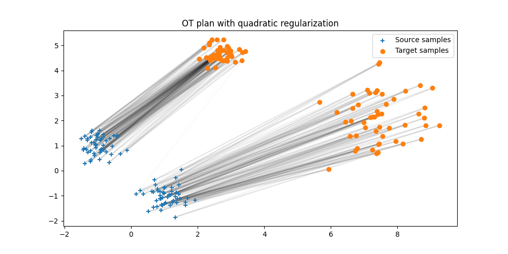
Text(0.5, 1.0, 'OT plan with quadratic regularization')