Sliced Wasserstein Distance with input scaling (DataScaler)

Note

Example added in release: 0.9.7.

This example illustrates why input scaling matters when computing the Sliced Wasserstein Distance (SWD) between distributions whose features have very different magnitudes. Without scaling, the SWD is dominated by high-magnitude features and may miss meaningful differences in low-magnitude features.

The ot.utils.DataScaler class fits normalization statistics once on a representative sample and applies the same fixed transformation on every call. This is preferred over re-normalizing inside each SWD call because the transformation stays consistent across mini-batches during optimization.

# Author: Harguna Sood <harguna.sood@gmail.com>
#
# License: MIT License

import matplotlib.pylab as pl
import numpy as np

import ot

Generate two 2D distributions with mismatched feature scales

Feature 1 is on the scale of 1000 with random noise. Feature 2 is on the scale of 1 with a meaningful 5-sigma shift between source and target distributions.

rng = np.random.RandomState(0)
n = 500

X_s = np.column_stack(
    [
        rng.normal(1000, 100, n),  # feature 1: large scale, no real signal
        rng.normal(0, 1, n),  # feature 2: small scale, no shift
    ]
)
X_t = np.column_stack(
    [
        rng.normal(1000, 100, n),  # feature 1: same distribution as source
        rng.normal(5, 1, n),  # feature 2: shifted by 5 std
    ]
)

SWD without scaling

Because feature 1 has values ~1000x larger than feature 2, the random projections used in SWD are dominated by feature 1. The meaningful shift in feature 2 is buried.

swd_raw = ot.sliced_wasserstein_distance(X_s, X_t, n_projections=200, seed=0)
print("SWD without scaling: {:.4f}".format(swd_raw))

SWD without scaling: 7.2575

SWD with DataScaler

Fit a standard scaler jointly on both distributions, then pass it to SWD. The same fixed statistics are reused on every call, giving a stable loss across mini-batches.

scaler = ot.utils.DataScaler(norm="standard").fit([X_s, X_t])
swd_scaled = ot.sliced_wasserstein_distance(
    X_s, X_t, n_projections=200, seed=0, scaler=scaler
)
print("SWD with DataScaler: {:.4f}".format(swd_scaled))

SWD with DataScaler: 1.2826

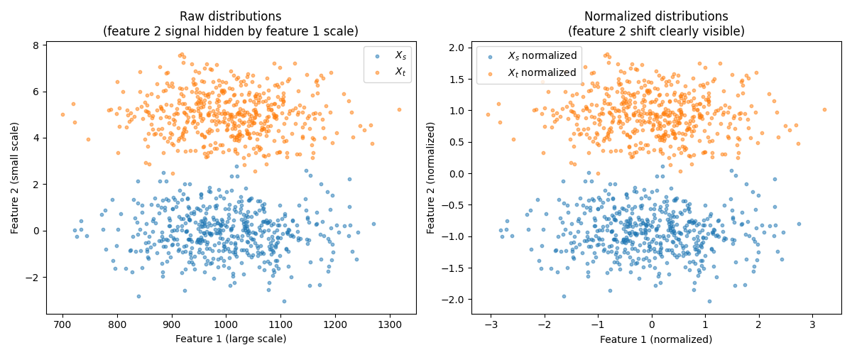
Visualize raw vs. scaled distributions

X_s_n = scaler.transform(X_s)
X_t_n = scaler.transform(X_t)

pl.figure(1, figsize=(12, 5))

pl.subplot(1, 2, 1)
pl.scatter(X_s[:, 0], X_s[:, 1], alpha=0.5, label="$X_s$", s=10)
pl.scatter(X_t[:, 0], X_t[:, 1], alpha=0.5, label="$X_t$", s=10)
pl.title("Raw distributions\n(feature 2 signal hidden by feature 1 scale)")
pl.xlabel("Feature 1 (large scale)")
pl.ylabel("Feature 2 (small scale)")
pl.legend()

pl.subplot(1, 2, 2)
pl.scatter(X_s_n[:, 0], X_s_n[:, 1], alpha=0.5, label="$X_s$ normalized", s=10)
pl.scatter(X_t_n[:, 0], X_t_n[:, 1], alpha=0.5, label="$X_t$ normalized", s=10)
pl.title("Normalized distributions\n(feature 2 shift clearly visible)")
pl.xlabel("Feature 1 (normalized)")
pl.ylabel("Feature 2 (normalized)")
pl.legend()

pl.tight_layout()
pl.show()